import hecfdapy as fda
import matplotlib.pyplot as plt
import numpy as npDistributions (Python)
hecfda’s C++ core ports all 13 distribution families from HEC.FDA.Statistics. Every family is addressed the same way: a name string and a numeric parameter list, in the order the core factory expects (the same order the fixtures/distributions/*.json oracle files use). One generic set of functions covers all of them: dist_pdf(), dist_cdf(), dist_quantile(), and dist_sample().
Nine families are reachable this way, through the generic factory dispatch:
| Family | Name string | Parameter order | Notes |
|---|---|---|---|
| Normal | "Normal" |
mean, sd, sample_size |
|
| Uniform | "Uniform" |
min, max, sample_size |
|
| Triangular | "Triangular" |
min, most_likely, max, sample_size |
|
| Deterministic | "Deterministic" |
value |
a point mass |
| LogNormal | "LogNormal" |
mean, sd, sample_size |
moments of the natural-log-scale data |
| TruncatedNormal | "TruncatedNormal" |
mean, sd, min, max, sample_size |
|
| TruncatedLogNormal | "TruncatedLogNormal" |
mean, sd, min, max, sample_size |
moments of the natural-log-scale data |
| LogPearsonIII | "LogPearsonIII" |
mean, sd, skew, sample_size |
moments of the log10-scale data; the flood-frequency workhorse |
| TruncatedLogPearson3 | "TruncatedLogPearson3" |
mean, sd, skew, min, max, sample_size |
moments of the log10-scale data |
Four of the 13 families are not on this list, and calling dist_pdf() with any of their names raises an error rather than constructing one. Gamma, ShiftedGamma, and PearsonIII are internal helper classes in the C++ core, not members of the IDistribution factory, so they have no name string at all. Empirical is a full IDistribution member, but is not constructible by name through the factory: it is built from data (a histogram or a set of quantiles), not from a short parameter list, so it has its own construction path rather than a dist_pdf()-style entry point. See the porting status page for where each of these lives.
Density, CDF, and quantile
Two families illustrate the range hecfda covers: Normal, a light-tailed, symmetric distribution, and LogPearsonIII, the heavy-tailed flood-frequency distribution HEC-FDA uses for annual peak flows. Both plots below evaluate dist_pdf(), dist_cdf(), and dist_quantile() over a grid and draw the three curves in the same earth-tone palette used throughout these examples.
x = np.linspace(-4, 4, 200)
p = np.linspace(0.001, 0.999, 200)
params = [0, 1, 1]

fig, axes = plt.subplots(1, 3, figsize=(9, 3))
axes[0].plot(x, fda.dist_pdf("Normal", params, x), color="#6b705c", linewidth=2)
axes[0].set(xlabel="x", ylabel="density", title="pdf")
axes[1].plot(x, fda.dist_cdf("Normal", params, x), color="#a5a58d", linewidth=2)
axes[1].set(xlabel="x", ylabel="probability", title="cdf")
axes[2].plot(p, fda.dist_quantile("Normal", params, p), color="#cb997e", linewidth=2)
axes[2].set(xlabel="probability", ylabel="x", title="quantile")
fig.suptitle("Normal(mean = 0, sd = 1)")
fig.tight_layout()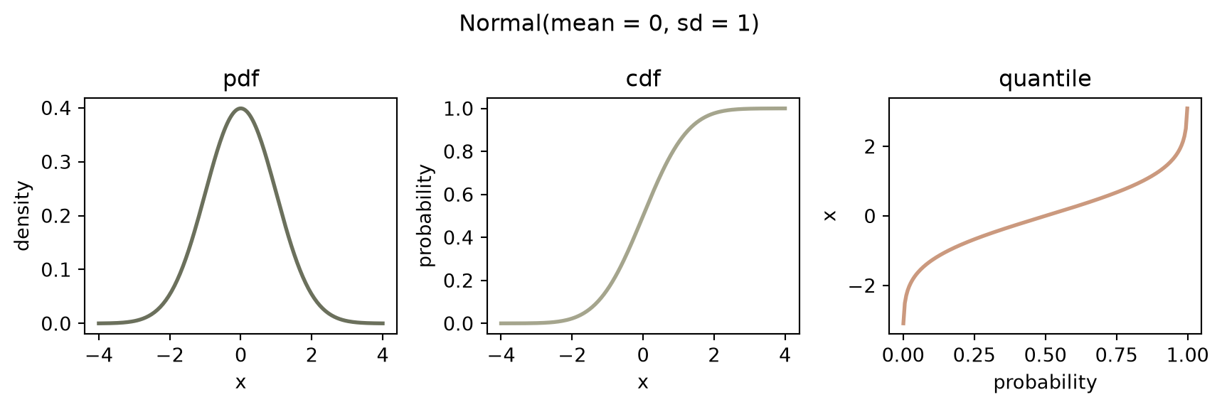
x = np.linspace(100, 12000, 200)
p = np.linspace(0.01, 0.99, 200)
params = [3.3, 0.254, 0.0925, 99]

fig, axes = plt.subplots(1, 3, figsize=(9, 3))
axes[0].plot(x, fda.dist_pdf("LogPearsonIII", params, x), color="#6b705c", linewidth=2)
axes[0].set(xlabel="x", ylabel="density", title="pdf")
axes[1].plot(x, fda.dist_cdf("LogPearsonIII", params, x), color="#a5a58d", linewidth=2)
axes[1].set(xlabel="x", ylabel="probability", title="cdf")
axes[2].plot(p, fda.dist_quantile("LogPearsonIII", params, p), color="#cb997e", linewidth=2)
axes[2].set(xlabel="probability", ylabel="x", title="quantile")
fig.suptitle("LogPearsonIII(mean = 3.3, sd = 0.254, skew = 0.0925, sample_size = 99)")
fig.tight_layout()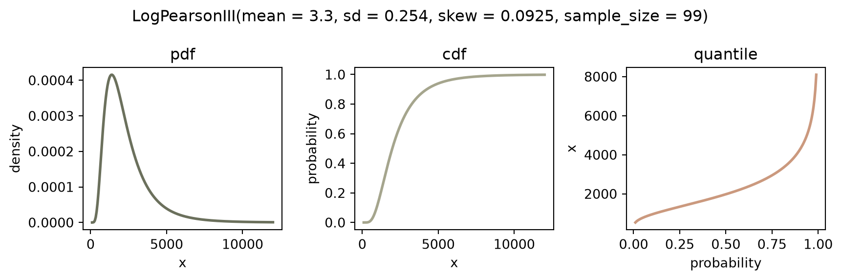
Seeded sampling
dist_sample() draws n values by applying the seeded generator’s uniform stream through inverse_cdf(), the same path every Monte Carlo compute in hecfda uses. A histogram of 1000 seeded Normal draws should track the analytic density closely:
draws = fda.dist_sample("Normal", [0, 1, 1], n=1000, seed=12345)

fig, ax = plt.subplots(figsize=(6, 4))
ax.hist(draws, bins=30, density=True, color="#a5a58d", edgecolor="white")
x = np.linspace(-4, 4, 200)
ax.plot(x, fda.dist_pdf("Normal", [0, 1, 1], x), color="#588157", linewidth=2)
ax.set(xlabel="x", ylabel="density")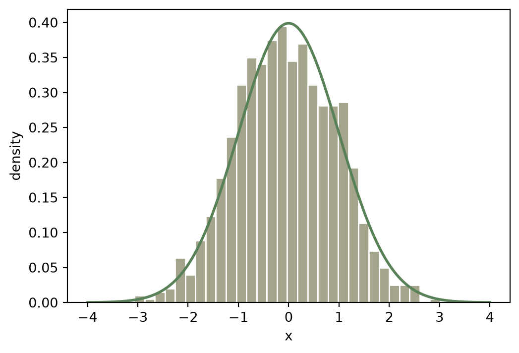
dist_sample("Normal", c(0, 1, 1), n = 1000L, seed = 12345L) in R draws the identical 1000 values, in the identical order, because both languages call the same seeded C++ generator.
Faithful bugs
Warning
This port reproduces upstream HEC-FDA behavior exactly, including a few known quirks in the C# source. Two examples that affect distributions:
Empirical’s pdf returns 0 for anyxthat is not an exact grid point in its data, rather than interpolating between points.LogNormalmixes natural-log (ln) andlog10semantics inconsistently between its methods, matching the same inconsistency in the C# source rather than normalizing it.
These are not bugs in the port; they are the upstream behavior, transcribed on purpose so results match HEC-FDA exactly. The porting status page describes what is ported and what was left out.