Stage-damage curves (R)

The problem

A stage-damage curve answers one question: for a given flood stage, how much dollar damage does a group of structures take? HEC-FDA builds that curve from three inputs – a structure inventory, a depth-percent-damage function per occupancy type, and the hydraulics that convert a flood event into a water-surface elevation at each structure – and adds a stage-frequency curve so the same compute can report damage against exceedance probability, not just stage.

This example rebuilds the upstream TractableStageDamageTests scenario: a simple two-structure Residential inventory where the answer is checkable by hand. It reproduces the published damage values for Residential/Structure at stages 12 through 19:

{0, 0, 30, 60, 90, 120, 150, 180}

The inventory

Two residential structures. Structure values are 100 and 200; first-floor elevations are 14 and 15; both sit on ground at elevation 12.

structures = data.frame(
  fid = c("1", "2"),
  first_floor_elevation = c(14, 15),
  value_structure = c(100, 200),
  damage_category = "Residential",
  occupancy_type = "Residential",
  ground_elevation = 12
)
structures

  fid first_floor_elevation value_structure damage_category occupancy_type
1   1                    14             100     Residential    Residential
2   2                    15             200     Residential    Residential
  ground_elevation
1               12
2               12

The occupancy type

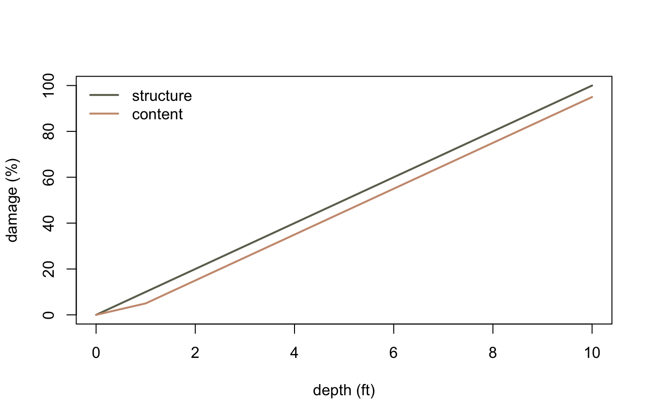
An occupancy type carries one depth-percent-damage curve per asset category. Here both curves are deterministic (no sampling uncertainty): structure damage rises linearly from 0% at depth 0 to 100% at depth 10, and content damage follows a similar rise scaled down slightly. A content-to-structure value ratio (CSVR) of 50 converts the content percentage into dollars from the same structure value.

depths = 0:10
struct_pct = seq(0, 100, by = 10)
content_pct = c(0, 5, 15, 25, 35, 45, 55, 65, 75, 85, 95)

occupancy_types = list(list(
  name = "Residential", damage_category = "Residential",
  structure_curve = list(x = depths, dist = "Deterministic", params = as.list(struct_pct)),
  content_curve = list(x = depths, dist = "Deterministic", params = as.list(content_pct)),
  content_to_structure_value_ratio = list(central = 50)
))

plot(depths, struct_pct, type = "l", col = "#6b705c", lwd = 2, ylim = c(0, 100),
     xlab = "depth (ft)", ylab = "damage (%)")
lines(depths, content_pct, col = "#cb997e", lwd = 2)
legend("topleft", legend = c("structure", "content"), col = c("#6b705c", "#cb997e"),
       lwd = 2, bty = "n")

Residential depth-percent-damage curves

Hydraulics and frequency

Eight exceedance probabilities drive the compute, from the common 0.5 event down to the rare 0.002 event. Each probability has a water-surface-elevation profile, one value per structure; here the profiles start at stages 13 and 14 for the two structures and rise by 1 ft per probability step. A graphical stage-frequency curve (stages 12 through 19, equivalent record length 50) lets the same compute report damage against frequency.

probabilities = c(.5, .2, .1, .04, .02, .01, .004, .002)
wses = Reduce(\(prev, i) prev + 1, seq_len(7), init = c(13, 14), accumulate = TRUE)

hydraulics = list(probabilities = probabilities, wses = wses)
stage_frequency = list(probabilities = probabilities, stages = 12:19, erl = 50)

Compute and compare

res = stage_damage(
  structures, occupancy_types, hydraulics, stage_frequency,
  stages = 12:19, impact_area_id = 34
)
structure_damage = res[res$damage_category == "Residential" & res$asset_category == "Structure", ]
structure_damage

  damage_category asset_category stage damage
1     Residential      Structure    12      0
2     Residential      Structure    13      0
3     Residential      Structure    14     30
4     Residential      Structure    15     60
5     Residential      Structure    16     90
6     Residential      Structure    17    120
7     Residential      Structure    18    150
8     Residential      Structure    19    180

plot(structure_damage$stage, structure_damage$damage, type = "b", col = "#588157", lwd = 2,
     pch = 16, xlab = "stage (ft)", ylab = "damage ($)")

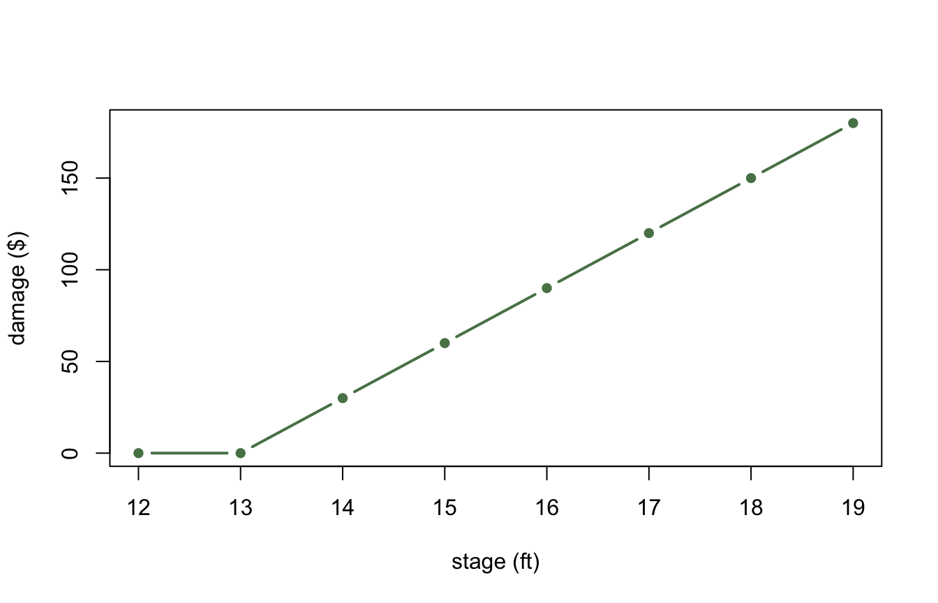
Residential/Structure stage-damage curve

The upstream oracle for Residential/Structure at stages 12-19 is {0, 0, 30, 60, 90, 120, 150, 180}. The computed values line up exactly:

data.frame(
  stage = structure_damage$stage,
  computed = structure_damage$damage,
  oracle = c(0, 0, 30, 60, 90, 120, 150, 180)
)

  stage computed oracle
1    12        0      0
2    13        0      0
3    14       30     30
4    15       60     60
5    16       90     90
6    17      120    120
7    18      150    150
8    19      180    180

Why the numbers are trustworthy

This scenario is not a made-up smoke test. It is the exact TractableStageDamageTests case from the upstream HEC-FDA C# source, and the dotnet oracle gate (make oracles) replays it against the real HEC.FDA.Model.ImpactAreaStageDamage.Compute and checks that this port’s output reproduces it to tolerance. The Compute call above runs the same convergence loop as production HEC-FDA; on this deterministic scenario it converges after the first chunk, but the loop, the consequence binning, and the curve construction are the same code the seeded Monte Carlo examples use.