import hecfdapy as fda
import pandas as pd
import matplotlib.pyplot as pltStage-damage curves (Python)
The problem
A stage-damage curve answers one question: for a given flood stage, how much dollar damage does a group of structures take? HEC-FDA builds that curve from three inputs – a structure inventory, a depth-percent-damage function per occupancy type, and the hydraulics that convert a flood event into a water-surface elevation at each structure – and adds a stage-frequency curve so the same compute can report damage against exceedance probability, not just stage.
This example rebuilds the upstream TractableStageDamageTests scenario: a simple two-structure Residential inventory where the answer is checkable by hand. It reproduces the published damage values for Residential/Structure at stages 12 through 19:
{0, 0, 30, 60, 90, 120, 150, 180}The inventory
Two residential structures. Structure values are 100 and 200; first-floor elevations are 14 and 15; both sit on ground at elevation 12.
structures = pd.DataFrame({
    "fid": ["1", "2"],
    "first_floor_elevation": [14, 15],
    "value_structure": [100, 200],
    "damage_category": ["Residential", "Residential"],
    "occupancy_type": ["Residential", "Residential"],
    "ground_elevation": [12, 12],
})
structures| fid | first_floor_elevation | value_structure | damage_category | occupancy_type | ground_elevation | |
|---|---|---|---|---|---|---|
| 0 | 1 | 14 | 100 | Residential | Residential | 12 |
| 1 | 2 | 15 | 200 | Residential | Residential | 12 |
The occupancy type
An occupancy type carries one depth-percent-damage curve per asset category. Here both curves are deterministic (no sampling uncertainty): structure damage rises linearly from 0% at depth 0 to 100% at depth 10, and content damage follows a similar rise scaled down slightly. A content-to-structure value ratio (CSVR) of 50 converts the content percentage into dollars from the same structure value.
depths = list(range(11))
struct_pct = [10 * i for i in range(11)]
content_pct = [0, 5, 15, 25, 35, 45, 55, 65, 75, 85, 95]

occupancy_types = [{
    "name": "Residential", "damage_category": "Residential",
    "structure_curve": {"x": depths, "dist": "Deterministic",
                        "params": [[v] for v in struct_pct]},
    "content_curve": {"x": depths, "dist": "Deterministic",
                      "params": [[v] for v in content_pct]},
    "content_to_structure_value_ratio": {"central": 50},
}]
fig, ax = plt.subplots(figsize=(6, 4))
ax.plot(depths, struct_pct, color="#6b705c", linewidth=2, label="structure")
ax.plot(depths, content_pct, color="#cb997e", linewidth=2, label="content")
ax.set(xlabel="depth (ft)", ylabel="damage (%)")
ax.legend(frameon=False)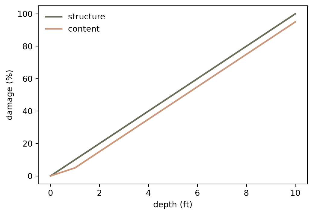
Hydraulics and frequency
Eight exceedance probabilities drive the compute, from the common 0.5 event down to the rare 0.002 event. Each probability has a water-surface-elevation profile, one value per structure; here the profiles start at stages 13 and 14 for the two structures and rise by 1 ft per probability step. A graphical stage-frequency curve (stages 12 through 19, equivalent record length 50) lets the same compute report damage against frequency.
probabilities = [.5, .2, .1, .04, .02, .01, .004, .002]
wses = [[13, 14]]
for _ in range(7):
    wses.append([w + 1 for w in wses[-1]])

hydraulics = {"probabilities": probabilities, "wses": wses}
stage_frequency = {"probabilities": probabilities, "stages": list(range(12, 20)), "erl": 50}
Compute and compare
res = fda.stage_damage(
    structures, occupancy_types, hydraulics, stage_frequency,
    stages=list(range(12, 20)), impact_area_id=34,
)
res_df = pd.DataFrame(res)
structure_damage = res_df[
    (res_df["damage_category"] == "Residential") & (res_df["asset_category"] == "Structure")
]
structure_damage| damage_category | asset_category | stage | damage | |
|---|---|---|---|---|
| 0 | Residential | Structure | 12.0 | 0.0 |
| 1 | Residential | Structure | 13.0 | 0.0 |
| 2 | Residential | Structure | 14.0 | 30.0 |
| 3 | Residential | Structure | 15.0 | 60.0 |
| 4 | Residential | Structure | 16.0 | 90.0 |
| 5 | Residential | Structure | 17.0 | 120.0 |
| 6 | Residential | Structure | 18.0 | 150.0 |
| 7 | Residential | Structure | 19.0 | 180.0 |
fig, ax = plt.subplots(figsize=(6, 4))
ax.plot(structure_damage["stage"], structure_damage["damage"], color="#588157", linewidth=2,
        marker="o")
ax.set(xlabel="stage (ft)", ylabel="damage ($)")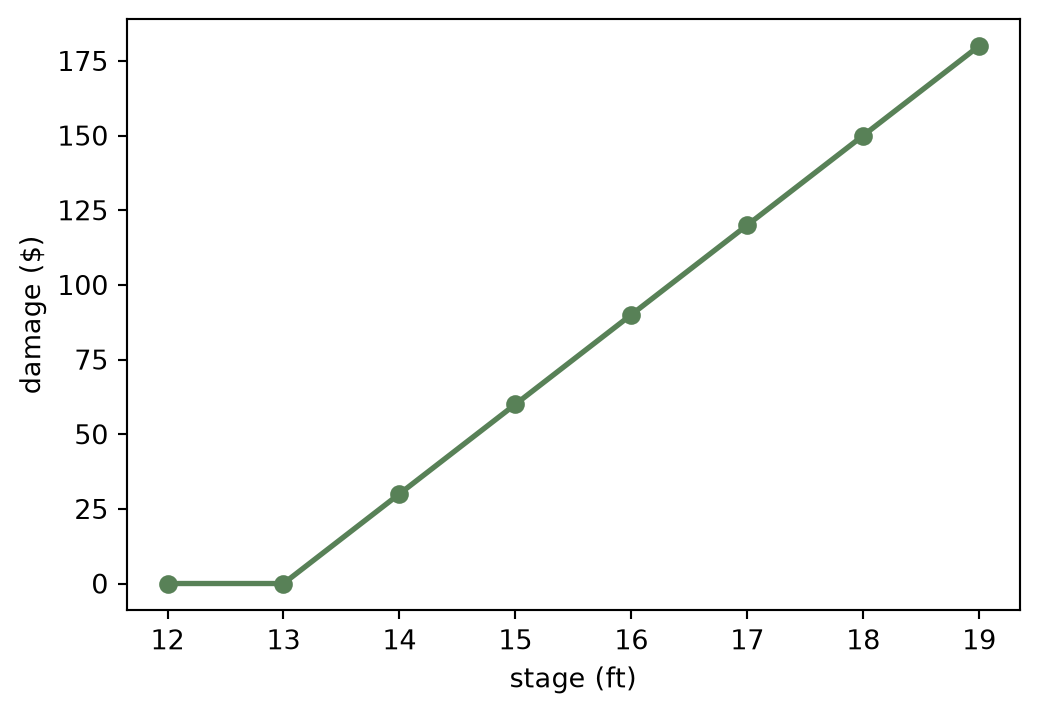
The upstream oracle for Residential/Structure at stages 12-19 is {0, 0, 30, 60, 90, 120, 150, 180}. The computed values line up exactly:
pd.DataFrame({
    "stage": structure_damage["stage"].to_numpy(),
    "computed": structure_damage["damage"].to_numpy(),
    "oracle": [0, 0, 30, 60, 90, 120, 150, 180],
})| stage | computed | oracle | |
|---|---|---|---|
| 0 | 12.0 | 0.0 | 0 |
| 1 | 13.0 | 0.0 | 0 |
| 2 | 14.0 | 30.0 | 30 |
| 3 | 15.0 | 60.0 | 60 |
| 4 | 16.0 | 90.0 | 90 |
| 5 | 17.0 | 120.0 | 120 |
| 6 | 18.0 | 150.0 | 150 |
| 7 | 19.0 | 180.0 | 180 |
Why the numbers are trustworthy
This scenario is not a made-up smoke test. It is the exact TractableStageDamageTests case from the upstream HEC-FDA C# source, and the dotnet oracle gate (make oracles) replays it against the real HEC.FDA.Model.ImpactAreaStageDamage.Compute and checks that this port’s output reproduces it to tolerance. The stage_damage call above runs the same convergence loop as production HEC-FDA; on this deterministic scenario it converges after the first chunk, but the loop, the consequence binning, and the curve construction are the same code the seeded Monte Carlo examples use.