EAD simulation (Python)

import math
import hecfdapy as fda
import matplotlib.pyplot as plt

The problem

Expected annual damage (EAD) is HEC-FDA’s core risk metric: expected dollar damage per year, integrated over every flood event weighted by how often it happens. The compute chains four pieces together:

A frequency curve – how often a flood of a given size occurs (an exceedance probability for each flow).
A flow-stage (rating) curve – converts flow to a water-surface stage.
One or more stage-damage curves – convert stage to dollar damage, per damage category and asset category.
An integration step – combines damage and frequency across the whole curve into EAD.

Every point on every curve can carry sampling uncertainty (a distribution instead of a fixed number). ead_simulation() runs this as a seeded Monte Carlo: draw once from each distribution, walk the four steps, accumulate the result into a histogram, repeat, report the mean. With deterministic=True and a single iteration, every distribution collapses to its mean instead of sampling, so what’s left is the plain arithmetic of the pipeline with no Monte Carlo noise at all.

This is the same construct as the getting-started example, spelled out properly this time: a Uniform(0, 100000) flow frequency, a flow-stage line from (0, 0) to (100000, 30), and a stage-damage curve that is flat at 600000 for any stage of 15 or more.

sim = dict(
    flow_frequency=dict(dist="Uniform", params=[0, 100000, 1000]),
    flow_stage=dict(x=[0, 100000], dist="Uniform", params=[[0, 0, 10], [0, 30, 10]]),
    stage_damage=[dict(
        x=[0, 15, 30], dist="Uniform",
        params=[[0, 0, 10], [0, 600000, 10], [0, 600000, 10]],
        damage_category="residential", asset_category="Structure",
    )],
)

res = fda.ead_simulation(**sim, min_iterations=1, max_iterations=1, deterministic=True)
res["total_ead"], res["mean_aep"]

(149999.99849999996, 0.9505)

res["total_ead"] is 150000 – the HEC-FDA deterministic oracle for this construct. res["mean_aep"] is the mean annual exceedance probability of the automatically-selected default performance threshold (HEC-FDA always derives one from the damage-frequency function itself, even with no threshold supplied): here it comes out to about 0.95, meaning this pipeline’s own damage-producing range is exceeded in most years.

A levee

A levee adds a fragility curve: the probability the levee fails, as a function of stage. Here the fragility is deterministic and binary – 0% failure probability below stage 9.9999, 100% failure probability at stage 10 and above – plus a top_of_levee_elevation marking where the levee itself sits.

sim_levee = dict(sim, levee=dict(
    x=[0, 9.9999, 10], dist="Deterministic", params=[[0], [0], [1]],
    damage_category="residential", asset_category="Structure",
    top_of_levee_elevation=100000,
))

res_levee = fda.ead_simulation(**sim_levee, min_iterations=1, max_iterations=1, deterministic=True)
res_levee["total_ead"]

84187.49849999994

Adding the levee cuts expected annual damage from 150000 to 84187.50 – HEC-FDA’s own oracle for this exact construct. The levee doesn’t erase damage: it only holds up to its own fragility curve, so above stage 10 damage still accrues at full risk. Below that, damage the base construct would have counted is now prevented.

Failure and non-failure damage

HEC-FDA 2.1 keeps damage during failure and non-failure states as separate rows. This deterministic levee case uses the same stage-damage curve in both roles. The system response and its complement partition the curve, so the two rows must sum to total EAD.

risk_curve = dict(
    x=[10, 11, 13, 17, 17.5], dist="Deterministic",
    params=[[0], [6000], [14000], [150000], [500000]],
    damage_category="residential", asset_category="Structure",
)
risk_sim = dict(
    flow_frequency=dict(dist="Uniform", params=[0, 1000, 5]),
    flow_stage=dict(
        x=[0, 250, 500, 750, 1000], dist="Deterministic",
        params=[[10], [11], [13], [17], [17.5]],
    ),
    stage_damage=[risk_curve],
    non_failure_stage_damage=[risk_curve],
    levee=dict(
        x=[10, 11, 13, 17, 17.5], dist="Deterministic",
        params=[[0], [0], [0.1], [0.8], [1]],
        damage_category="residential", asset_category="Structure",
        top_of_levee_elevation=17,
    ),
)
risk_result = fda.ead_simulation(
    **risk_sim, min_iterations=1, max_iterations=1, deterministic=True
)
risk_result["ead_by_risk"]

[{'damage_category': 'residential',
  'asset_category': 'Structure',
  'risk_type': 'Fail',
  'mean_ead': 92849.99239999993},
 {'damage_category': 'residential',
  'asset_category': 'Structure',
  'risk_type': 'Non_Fail',
  'mean_ead': 12150.000599999996}]

assert [row["risk_type"] for row in risk_result["ead_by_risk"]] == [
    "Fail", "Non_Fail"
]
assert math.isclose(
    risk_result["total_ead"],
    sum(row["mean_ead"] for row in risk_result["ead_by_risk"]),
)

The ordered rows reproduce the shared v2.1 fixture: failure EAD is about 92849.99, non-failure EAD is about 12150.00, and their sum is about 104999.99. Total is the aggregate query used to obtain that sum, not a third stored row.

The seeded Monte Carlo

Switch deterministic off and every distribution samples instead of collapsing to its mean. Each curve draws from HEC-FDA’s own seeded generator with a fixed constant per curve type – frequency 1234, flow-stage 3456, stage-damage 6789, and four more for interior/exterior stage, system response, and life loss – ported exactly from the C# source. The exact sequence of draws, and so the exact result, is reproducible across runs, across languages, and against the real HEC-FDA.

The fixture this example reproduces also tags the flow-stage curve with the same damage and asset category as the stage-damage curve; the seeded compute’s random-number setup needs that tag to line up (the deterministic pass above works without it):

sim = dict(sim, flow_stage=dict(sim["flow_stage"], damage_category="residential",
                                asset_category="Structure"))

res_100 = fda.ead_simulation(**sim, min_iterations=100, max_iterations=100, deterministic=False)
res_100["total_ead"]

121194.5159789352

At exactly 100 iterations this is 121194.5159789352 – bit-for-bit the number the real HEC-FDA C# produces at the same iteration count, in both R and Python. That’s the strongest check a Monte Carlo port can offer: not that two implementations land close together by chance, but that they draw the same sequence of random numbers and accumulate them the same way, all the way through the frequency -> stage -> damage -> integrate pipeline.

Convergence

Run the same construct at increasing iteration counts and watch the seeded mean settle toward its own limit:

iters = [100, 1000, 10000]
mean_ead = []
for n in iters:
    res_n = fda.ead_simulation(**sim, min_iterations=n, max_iterations=n, deterministic=False)
    mean_ead.append(res_n["total_ead"])

list(zip(iters, mean_ead))

[(100, 121194.5159789352),
 (1000, 133985.40478349788),
 (10000, 135275.88477692605)]

fig, ax = plt.subplots(figsize=(6, 4))
ax.plot(iters, mean_ead, color="#588157", linewidth=2, marker="o", label="seeded Monte Carlo")
ax.axhline(150000, color="#cb997e", linestyle="--", linewidth=2, label="deterministic (150000, reference only)")
ax.set_xscale("log")
ax.set(xlabel="iterations", ylabel="mean EAD ($)")
ax.legend(frameon=False)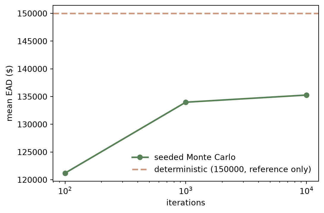

The sweep flattens near 135600, not 150000. That gap is not sampling noise, and more iterations will not close it. deterministic=True collapses every input distribution to its mean before any curve runs, so the deterministic pass evaluates the pipeline once on those mean values. The seeded Monte Carlo does the opposite: it samples first and evaluates the curves per draw, then averages the results. The stage-damage curve is nonlinear – flat at 600000 for any stage of 15 or more – so the mean of the damage is not the damage of the mean: E[f(X)] != f(E[X]). Averaging before a nonlinear curve and averaging after it are different questions with different correct answers. 150000 is the deterministic answer; the Monte Carlo converges to its own limit near 135600, and both are right.

Why the numbers are trustworthy

None of these values are made up. 150000, 84187.50, and 121194.5159789352 are the same literals the dotnet oracle gate (make oracles) checks against the real HEC.FDA.Model.ImpactAreaScenarioSimulation.Compute, and the last one is not just close: it is the exact value after exactly 100 iterations of the seeded Monte Carlo loop, reproduced bit-for-bit because the seven per-curve seed constants are ported exactly from the C# source, and every arithmetic step downstream of them matches too.