01. Probability distributions

Language: R (Quarto) - Python version

Ported from 01_distributions.ipynb in the USACE-RMC Numerics-Python-Examples repository (0BSD licensed). The upstream notebook drives the C# Numerics.dll through pythonnet; this version uses corehydror, whose compiled core is a validated C++ port of the same library, so the numbers below reproduce the upstream outputs exactly. The Python version of this example uses the same core and prints the same numbers.

What you’ll learn

Creating and parameterizing distributions by family name.
Computing PDF, CDF, and quantile values.
Statistical properties (mean, variance, skewness, kurtosis).
When to use each distribution.
Random sampling, including Latin hypercube sampling.

The upstream notebook tours ten of the 42 univariate families in the library: Normal, Log-Normal, GEV, Gamma, Weibull, Uniform, Triangular, PERT, Poisson, and Binomial. This port keeps every family and condenses the long mathematical derivations; see the upstream notebook for the full detail.

Setup

The upstream setup loads the CoreCLR runtime and imports each distribution class from Numerics.Distributions. Here one library() call covers everything, and every family is constructed by name through distribution().

library(corehydror)

# Earth-tone palette used throughout
olive <- "#6b7f3f"
clay <- "#b06a3b"
slate <- "#5b7a8c"
gray <- "#8c8c7a"

cat("Setup complete\n")

Setup complete

Basic example: the Normal distribution

The Normal (Gaussian) distribution is the most widely used continuous distribution. It arises naturally from the Central Limit Theorem: the sum of many independent random variables tends toward a Normal distribution regardless of the underlying distributions. It is parameterized by its mean \(\mu\) and standard deviation \(\sigma\):

\[ f(x) = \frac{1}{\sigma\sqrt{2\pi}} \exp\!\left(-\frac{(x - \mu)^2}{2\sigma^2}\right), \quad -\infty < x < \infty \]

Note that the library reports Pearson (non-excess) kurtosis, which is 3.0 for a Normal distribution. The “excess kurtosis” convention is Pearson minus 3.

When to use: symmetric data, many natural phenomena, Central Limit Theorem applications.

# Create Normal distribution -- Normal(mean = 100, sd = 15)
normal <- distribution("Normal", c(100, 15))
m <- dist_moments(normal)

cat("Mean:", m[["mean"]], "\n")

Mean: 100

cat("Standard Deviation:", m[["sd"]], "\n")

Standard Deviation: 15

cat("Variance:", m[["sd"]]^2, "\n")

Variance: 225

cat("Skewness:", m[["skewness"]], "\n")

Skewness: 0

cat("Kurtosis:", m[["kurtosis"]], "\n")

Kurtosis: 3

cat("Minimum:", m[["minimum"]], "\n")

Minimum: -Inf

cat("Maximum:", m[["maximum"]], "\n")

Maximum: Inf

cat("5th Percentile:", format(dist_quantile(normal, 0.05), digits = 17), "\n")

5th Percentile: 75.327195595727915

cat("Median:", dist_quantile(normal, 0.5), "\n")

Median: 100

cat("95th Percentile:", format(dist_quantile(normal, 0.95), digits = 17), "\n")

95th Percentile: 124.67280440427207

# Plot the PDF and CDF over the 0.1% to 99.9% quantile range.
# dist_pdf/dist_cdf/dist_quantile are all vectorized.
x <- seq(dist_quantile(normal, 0.001), dist_quantile(normal, 0.999),
         length.out = 500)

plot(x, dist_pdf(normal, x), type = "l", col = olive, lwd = 2,
     xlab = "x", ylab = "PDF", main = "Probability density function")
polygon(c(x, rev(x)), c(dist_pdf(normal, x), rep(0, length(x))),
        col = adjustcolor(olive, alpha.f = 0.25), border = NA)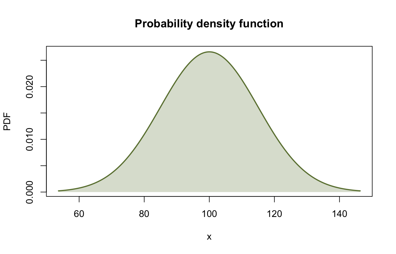

plot(x, dist_cdf(normal, x), type = "l", col = clay, lwd = 2,
     xlab = "x", ylab = "CDF", main = "Cumulative distribution function")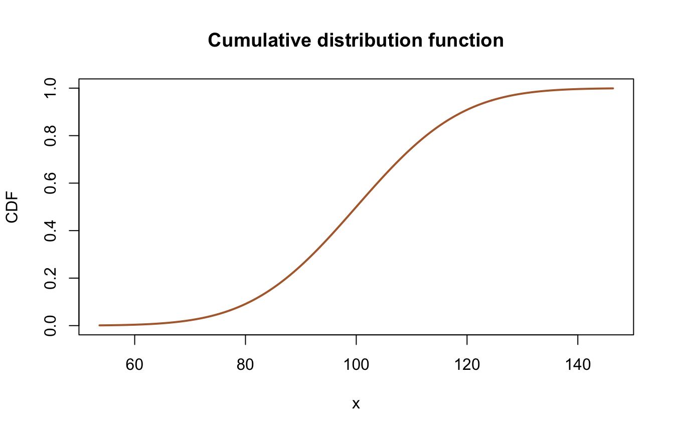

Helper functions

Two small helpers make the rest of the tour concise: one plots the PDF and CDF side by side, the other prints the statistics table the upstream notebook shows for each family.

plot_distribution <- function(dist, x_range = NULL, n_points = 500,
                              title = NULL) {
  # Plot PDF and CDF of a distribution.
  if (is.null(x_range)) {
    x_range <- dist_quantile(dist, c(0.001, 0.999))
  }
  x <- seq(x_range[1], x_range[2], length.out = n_points)
  op <- par(mfrow = c(1, 2))
  plot(x, dist_pdf(dist, x), type = "l", col = olive, lwd = 2,
       xlab = "x", ylab = "PDF", main = title)
  polygon(c(x, rev(x)), c(dist_pdf(dist, x), rep(0, length(x))),
          col = adjustcolor(olive, alpha.f = 0.25), border = NA)
  plot(x, dist_cdf(dist, x), type = "l", col = clay, lwd = 2,
       xlab = "x", ylab = "CDF")
  par(op)
}

print_statistics <- function(dist, name = "Distribution") {
  # Print the statistics table upstream shows for each family.
  m <- dist_moments(dist)
  q <- dist_quantile(dist, c(0.05, 0.5, 0.95))
  df <- data.frame(
    Statistic = c("Mean", "Std Deviation", "Variance", "Skewness",
                  "Kurtosis", "Minimum", "Maximum", "5th Percentile",
                  "Median", "95th Percentile"),
    Value = round(c(m[["mean"]], m[["sd"]], m[["sd"]]^2, m[["skewness"]],
                    m[["kurtosis"]], m[["minimum"]], m[["maximum"]], q), 4)
  )
  cat("\n", name, " statistics:\n", sep = "")
  print(df, row.names = FALSE)
}

Continuous distributions

A parameterization note before the tour: the library uses its own parameter conventions (for example, GEV uses \(\xi\), \(\alpha\), \(\kappa\) in the Hosking convention). If you compare to textbooks or other R packages, double-check the parameter definitions. dist_params(d) shows the constructor order for any family.

Log-Normal

A random variable \(X\) follows a Log-Normal distribution if \(\log(X)\) follows a Normal distribution. It suits strictly positive, right-skewed data arising from multiplicative processes. Matching the C# library, the "LogNormal" family uses base-10 logarithms: the parameters are the mean and standard deviation of \(\log_{10}(X)\). The upstream C# class has a mutable Base property; that is not exposed here. Use the "LnNormal" family when you want the base-\(e\) form.

When to use: right-skewed data that is always positive (flows, particle sizes, incomes).

lognormal <- distribution("LogNormal", c(4.0, 0.5))

print_statistics(lognormal, "LogNormal(4.0, 0.5)")


LogNormal(4.0, 0.5) statistics:
       Statistic        Value
            Mean 1.940096e+04
   Std Deviation 3.225447e+04
        Variance 1.040351e+09
        Skewness 9.582700e+00
        Kurtosis 3.468718e+02
         Minimum 0.000000e+00
         Maximum          Inf
  5th Percentile 1.505127e+03
          Median 1.000000e+04
 95th Percentile 6.643957e+04

plot_distribution(lognormal, title = "Log-Normal distribution")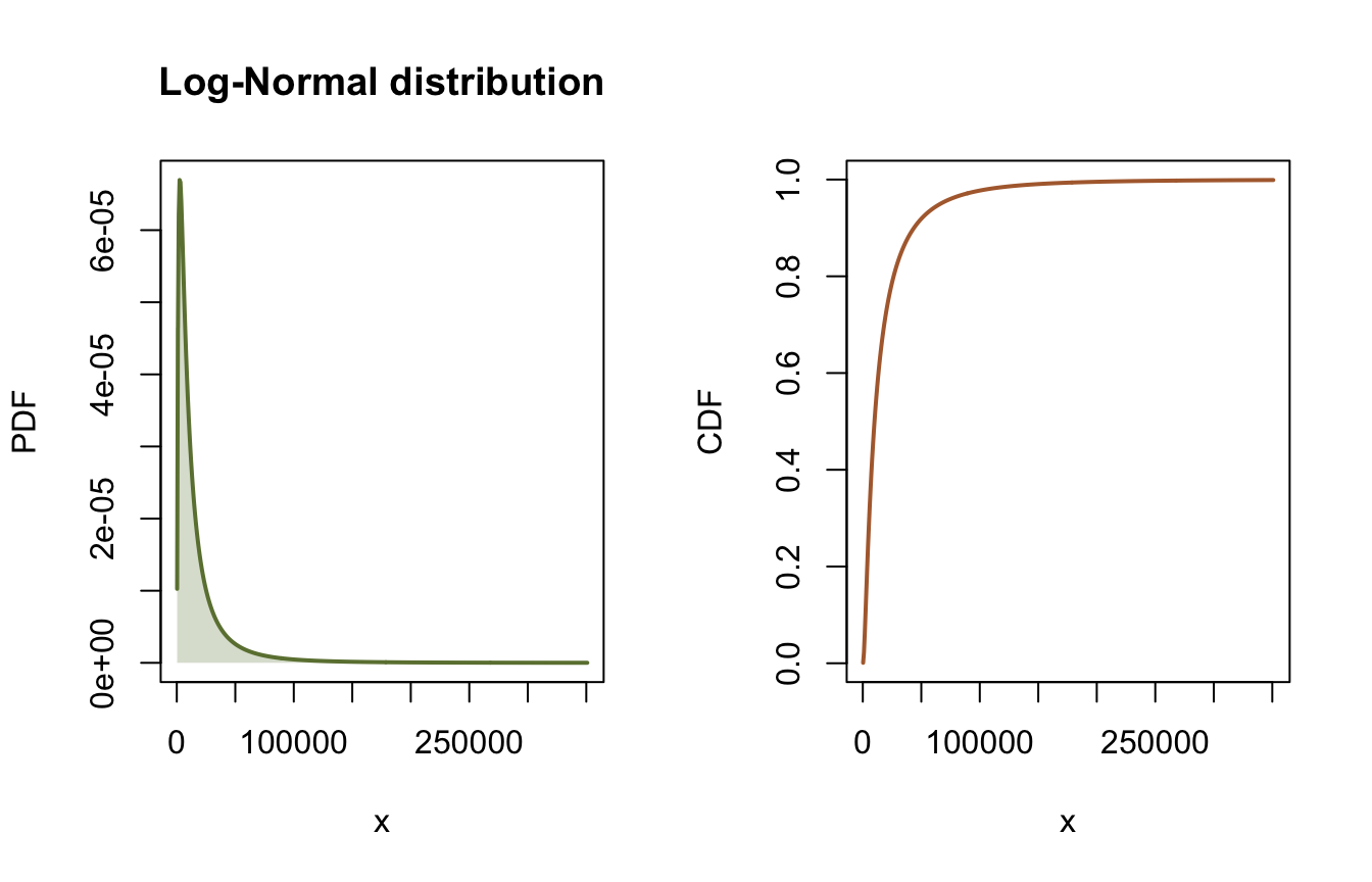

Generalized Extreme Value (GEV)

The GEV distribution unifies three classical extreme value distributions into a single three-parameter family. It is the limiting distribution for block maxima (annual maximum floods, peak wind speeds) under the Fisher-Tippett-Gnedenko theorem. The parameterization is location \(\xi\), scale \(\alpha > 0\), and shape \(\kappa\) in the Hosking convention, where the sign of \(\kappa\) follows L-moment theory:

\[ F(x) = \exp(-e^{-y}), \qquad y = \begin{cases} -\dfrac{1}{\kappa}\ln\!\left(1 - \kappa\dfrac{x - \xi}{\alpha}\right) & \kappa \neq 0 \\[6pt] \dfrac{x - \xi}{\alpha} & \kappa = 0 \end{cases} \]

\(\kappa < 0\): Frechet type (heavy upper tail, bounded below)
\(\kappa = 0\): Gumbel (unbounded)
\(\kappa > 0\): Weibull type (bounded above)

The mean exists when \(|\kappa| < 1\) and the variance when \(|\kappa| < 1/2\), which is why two of the three tables below show NaN moments.

When to use: extreme events (floods, droughts, maxima and minima).

# Hosking convention: kappa < 0 => Frechet; kappa > 0 => Weibull type
gev_frechet <- distribution("GeneralizedExtremeValue", c(100, 15, -0.5))
gev_gumbel <- distribution("GeneralizedExtremeValue", c(100, 15, 0.0))
gev_weibull <- distribution("GeneralizedExtremeValue", c(100, 15, 0.5))

x <- seq(50, 200, length.out = 500)
plot(x, dist_pdf(gev_frechet, x), type = "l", col = olive, lwd = 2,
     xlab = "x", ylab = "PDF", main = "GEV: effect of the shape parameter")
lines(x, dist_pdf(gev_gumbel, x), col = clay, lwd = 2)
lines(x, dist_pdf(gev_weibull, x), col = slate, lwd = 2)
legend("topright",
       legend = c("kappa = -0.5 (Frechet)", "kappa = 0.0 (Gumbel)",
                  "kappa = 0.5 (Weibull)"),
       col = c(olive, clay, slate), lwd = 2, bty = "n")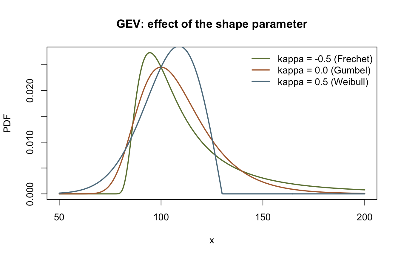

print_statistics(gev_frechet, "GEV (Frechet type)")


GEV (Frechet type) statistics:
       Statistic    Value
            Mean 123.1736
   Std Deviation      NaN
        Variance      NaN
        Skewness      NaN
        Kurtosis      NaN
         Minimum  70.0000
         Maximum      Inf
  5th Percentile  87.3328
          Median 106.0337
 95th Percentile 202.4619

print_statistics(gev_gumbel, "GEV (Gumbel type)")


GEV (Gumbel type) statistics:
       Statistic    Value
            Mean 108.6582
   Std Deviation  19.2382
        Variance 370.1102
        Skewness   1.1396
        Kurtosis   5.4000
         Minimum     -Inf
         Maximum      Inf
  5th Percentile  83.5422
          Median 105.4977
 95th Percentile 144.5529

print_statistics(gev_weibull, "GEV (Weibull type)")


GEV (Weibull type) statistics:
       Statistic    Value
            Mean 103.4132
   Std Deviation      NaN
        Variance      NaN
        Skewness      NaN
        Kurtosis      NaN
         Minimum     -Inf
         Maximum 130.0000
  5th Percentile  78.0754
          Median 105.0234
 95th Percentile 123.2056

Gamma

The Gamma distribution is a flexible two-parameter family for positive-valued data. It generalizes the Exponential distribution and appears in waiting-time problems, rainfall modeling, and Bayesian statistics. The factory name is "GammaDistribution" (matching the C# class name), with scale \(\theta\) first and shape \(\kappa\) second:

\[ f(x) = \frac{x^{\kappa-1}\, e^{-x/\theta}}{\theta^{\kappa}\,\Gamma(\kappa)}, \quad x > 0 \]

When to use: positive data, waiting times, rainfall amounts.

gamma_dist <- distribution("GammaDistribution", c(2.0, 0.5))
print_statistics(gamma_dist, "Gamma(scale=2, shape=0.5)")


Gamma(scale=2, shape=0.5) statistics:
       Statistic   Value
            Mean  1.0000
   Std Deviation  1.4142
        Variance  2.0000
        Skewness  2.8284
        Kurtosis 15.0000
         Minimum  0.0000
         Maximum     Inf
  5th Percentile  0.0039
          Median  0.4549
 95th Percentile  3.8415

plot_distribution(gamma_dist, x_range = c(0, 15), title = "Gamma distribution")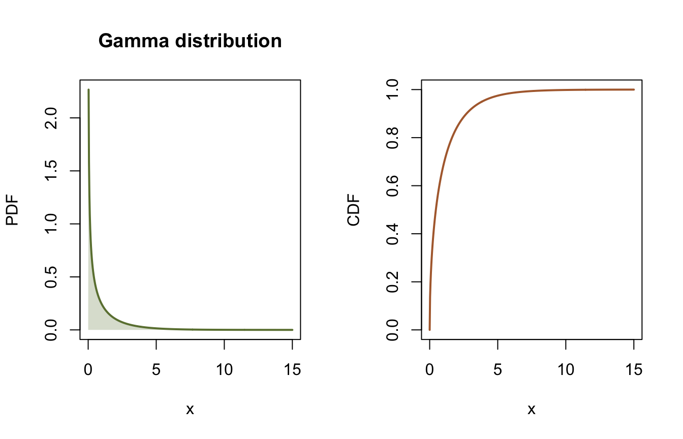

Weibull

The Weibull distribution is a flexible two-parameter model for nonnegative data. Its shape parameter controls the failure rate: \(\kappa < 1\) gives decreasing hazard (early failures), \(\kappa = 1\) reduces to the Exponential distribution, and \(\kappa > 1\) yields increasing hazard (wear-out):

\[ F(x) = 1 - \exp\left[-\left(\frac{x}{\lambda}\right)^{\kappa}\right], \quad x \ge 0 \]

When to use: reliability analysis, wind speeds, failure times.

weibull <- distribution("Weibull", c(100, 2.5))
print_statistics(weibull, "Weibull(scale=100, shape=2.5)")


Weibull(scale=100, shape=2.5) statistics:
       Statistic     Value
            Mean   88.7264
   Std Deviation   37.9667
        Variance 1441.4669
        Skewness    0.3586
        Kurtosis    2.8568
         Minimum    0.0000
         Maximum       Inf
  5th Percentile   30.4807
          Median   86.3635
 95th Percentile  155.0962

plot_distribution(weibull, x_range = c(0, 150), title = "Weibull distribution")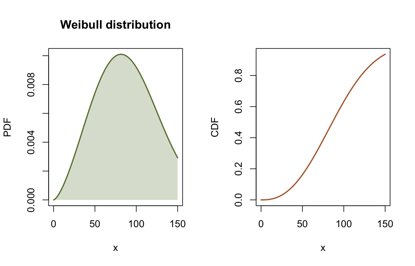

Bounded distributions

Three families for quantities with known bounds. The Uniform distribution assigns equal density to every value in \([a, b]\): maximum uncertainty given only the support. The Triangular distribution adds a most likely value (the mode) between the bounds, a common shape for expert elicitation. The PERT distribution (factory name "Pert") takes the same minimum, most likely, and maximum inputs but maps them to a smooth Beta density on \([a, b]\) with mean \((a + 4c + b)/6\), giving gentler tails than the Triangular.

When to use: bounded quantities; Uniform when only the range is known, Triangular or PERT when a most likely value is available (project estimates, expert opinion).

uniform <- distribution("Uniform", c(0, 100))
print_statistics(uniform, "Uniform(0, 100)")


Uniform(0, 100) statistics:
       Statistic    Value
            Mean  50.0000
   Std Deviation  28.8675
        Variance 833.3333
        Skewness   0.0000
        Kurtosis   1.8000
         Minimum   0.0000
         Maximum 100.0000
  5th Percentile   5.0000
          Median  50.0000
 95th Percentile  95.0000

plot_distribution(uniform, x_range = c(-10, 110), title = "Uniform(0, 100)")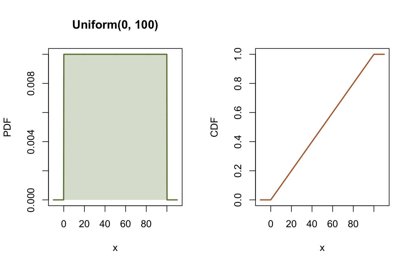

triangular <- distribution("Triangular", c(0, 30, 100))
print_statistics(triangular, "Triangular(0, 30, 100)")


Triangular(0, 30, 100) statistics:
       Statistic    Value
            Mean  43.3333
   Std Deviation  20.9497
        Variance 438.8889
        Skewness   0.3561
        Kurtosis   2.4000
         Minimum   0.0000
         Maximum 100.0000
  5th Percentile  12.2474
          Median  40.8392
 95th Percentile  81.2917

plot_distribution(triangular, x_range = c(-10, 110),
                  title = "Triangular(0, 30, 100)")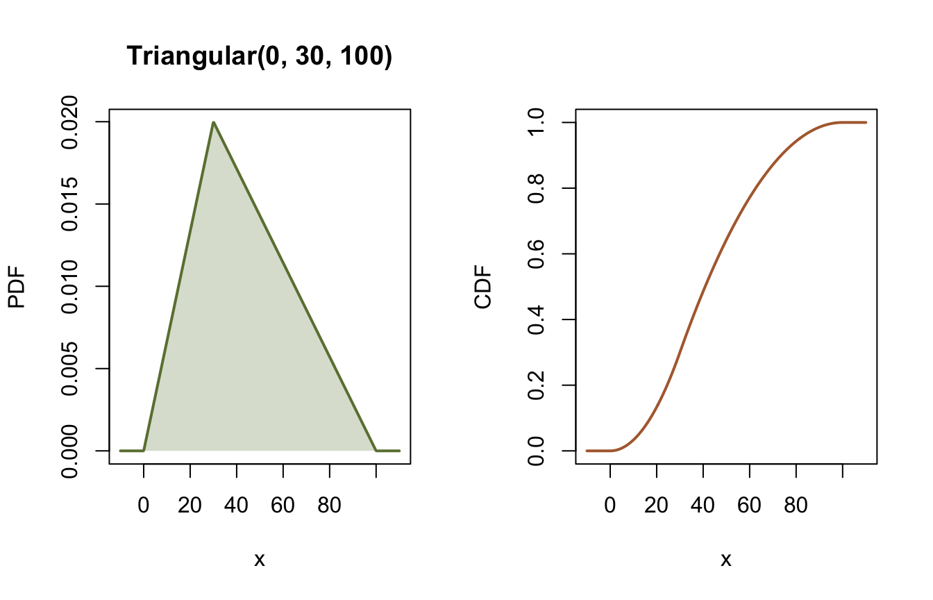

pert <- distribution("Pert", c(10, 50, 100))
print_statistics(pert, "PERT(10, 50, 100)")


PERT(10, 50, 100) statistics:
       Statistic    Value
            Mean  51.6667
   Std Deviation  16.9617
        Variance 287.6984
        Skewness   0.0983
        Kurtosis   2.3462
         Minimum  10.0000
         Maximum 100.0000
  5th Percentile  24.4643
          Median  51.2732
 95th Percentile  80.2234

# Compare PERT vs Triangular with the same min / most likely / max
tri <- distribution("Triangular", c(10, 50, 100))
x <- seq(5, 105, length.out = 500)
plot(x, dist_pdf(pert, x), type = "l", col = olive, lwd = 2,
     xlab = "x", ylab = "PDF", main = "PERT vs Triangular")
lines(x, dist_pdf(tri, x), col = clay, lwd = 2, lty = 2)
legend("topright", legend = c("PERT", "Triangular"),
       col = c(olive, clay), lwd = 2, lty = c(1, 2), bty = "n")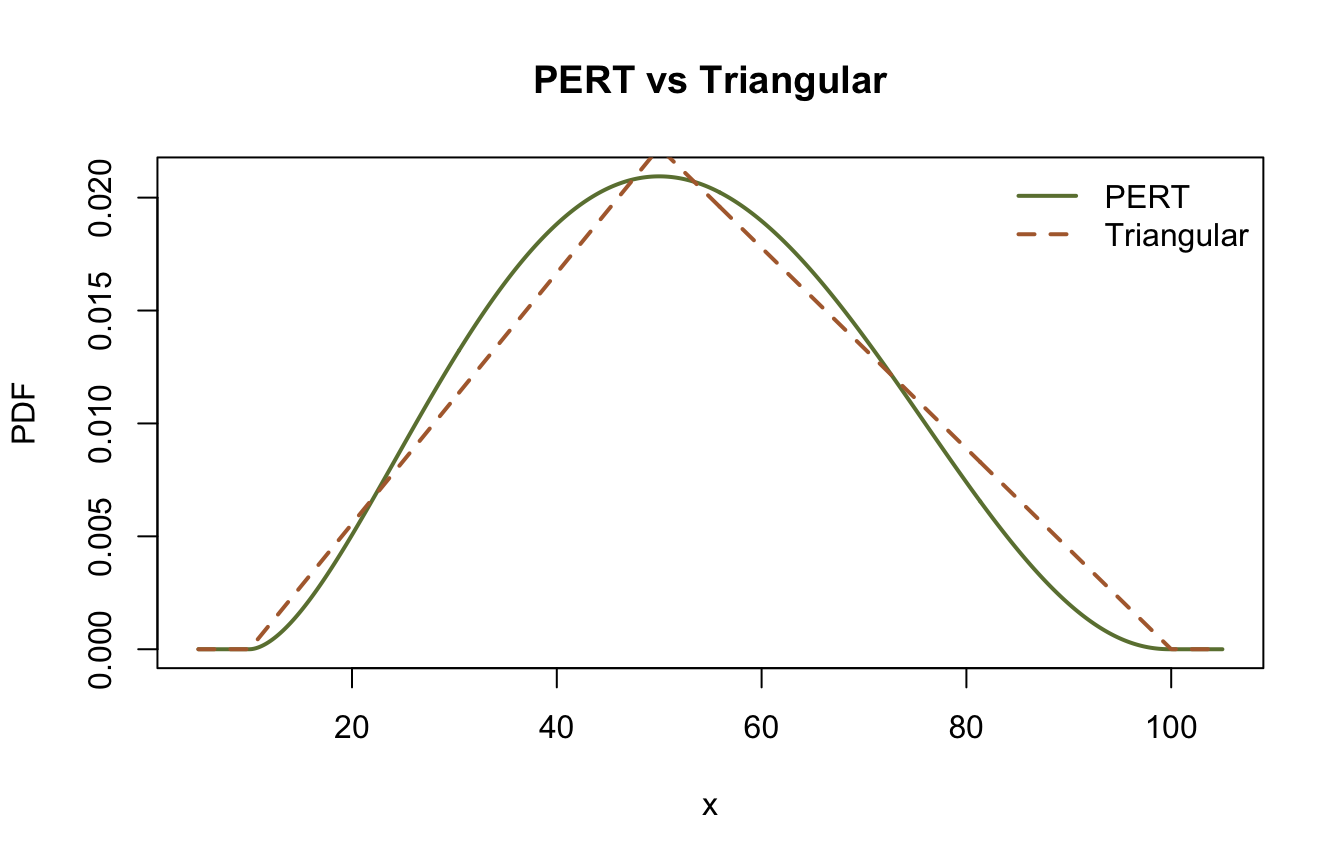

Discrete distributions

The library uses dist_pdf() for both continuous and discrete families; for discrete distributions, read dist_pdf() as the probability mass function (PMF).

Poisson

The Poisson distribution models counts of events over a fixed interval when events occur independently at a constant average rate \(\lambda\):

\[ P(X=k) = \frac{\lambda^{k} e^{-\lambda}}{k!}, \quad k = 0, 1, 2, \ldots \]

Mean and variance are both \(\lambda\).

When to use: count data, events per time period, rare events.

poisson <- distribution("Poisson", c(3.5))
print_statistics(poisson, "Poisson(3.5)")


Poisson(3.5) statistics:
       Statistic  Value
            Mean 3.5000
   Std Deviation 1.8708
        Variance 3.5000
        Skewness 0.5345
        Kurtosis 3.2857
         Minimum 0.0000
         Maximum    Inf
  5th Percentile 1.0000
          Median 3.0000
 95th Percentile 7.0000

k <- 0:14
op <- par(mfrow = c(1, 2))
barplot(dist_pdf(poisson, k), names.arg = k, col = olive, border = "white",
        xlab = "k (count)", ylab = "PMF")
plot(k, dist_cdf(poisson, k), type = "s", col = clay, lwd = 2,
     xlab = "k (count)", ylab = "CDF")
points(k, dist_cdf(poisson, k), col = clay, pch = 16, cex = 0.7)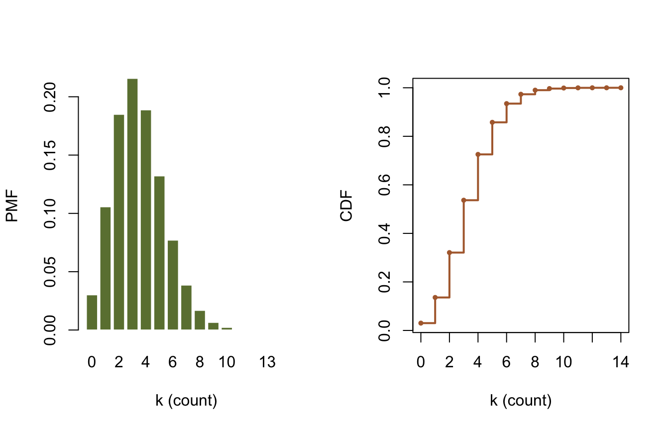

par(op)

cat(sprintf("P(X = 3): %.4f\n", dist_pdf(poisson, 3)))

P(X = 3): 0.2158

cat(sprintf("P(X <= 5): %.4f\n", dist_cdf(poisson, 5)))

P(X <= 5): 0.8576

Binomial

The Binomial distribution models the number of successes in \(n\) independent Bernoulli trials with success probability \(p\):

\[ P(X=k) = \binom{n}{k} p^k (1-p)^{n-k}, \quad k = 0, 1, \ldots, n \]

The constructor order matches the C# class: probability first, then the number of trials.

When to use: fixed number of trials with binary outcomes.

binomial <- distribution("Binomial", c(0.3, 20))
print_statistics(binomial, "Binomial(p=0.3, n=20)")


Binomial(p=0.3, n=20) statistics:
       Statistic   Value
            Mean  6.0000
   Std Deviation  2.0494
        Variance  4.2000
        Skewness  0.1952
        Kurtosis  2.9381
         Minimum  0.0000
         Maximum 20.0000
  5th Percentile  3.0000
          Median  6.0000
 95th Percentile  9.0000

k <- 0:20
barplot(dist_pdf(binomial, k), names.arg = k, col = olive, border = "white",
        xlab = "k (number of successes)", ylab = "PMF",
        main = "Binomial(p=0.3, n=20)")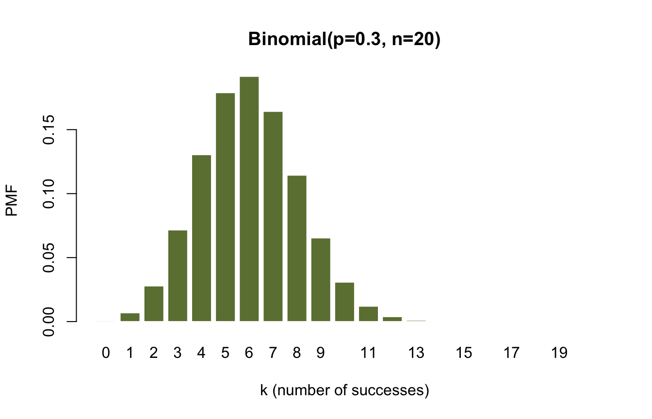

bm <- dist_moments(binomial)
cat(sprintf("Expected value: %.2f\n", bm[["mean"]]))

Expected value: 6.00

cat(sprintf("Most likely value: %d\n", as.integer(bm[["mean"]])))

Most likely value: 6

Generating and analyzing random samples

Every univariate distribution has a dist_random() method (the port of GenerateRandomValues). The upstream notebook draws these samples unseeded; here they are seeded so the histograms and the table below reproduce exactly, in both languages. The sample statistics therefore differ from the upstream run’s unseeded table, but match the Python version of this page bit for bit.

n_samples <- 10000

normal_samples <- dist_random(distribution("Normal", c(100, 15)),
                              n_samples, seed = 42)
lognormal_samples <- dist_random(distribution("LogNormal", c(4, 0.5)),
                                 n_samples, seed = 42)
gamma_samples <- dist_random(distribution("GammaDistribution", c(2, 0.5)),
                             n_samples, seed = 42)

op <- par(mfrow = c(1, 3))
hist(normal_samples, breaks = 50, freq = FALSE, col = olive, border = "white",
     main = "Normal", xlab = "Value")
hist(lognormal_samples, breaks = 50, freq = FALSE, col = olive,
     border = "white", main = "Log-Normal", xlab = "Value")
hist(gamma_samples, breaks = 50, freq = FALSE, col = olive, border = "white",
     main = "Gamma", xlab = "Value")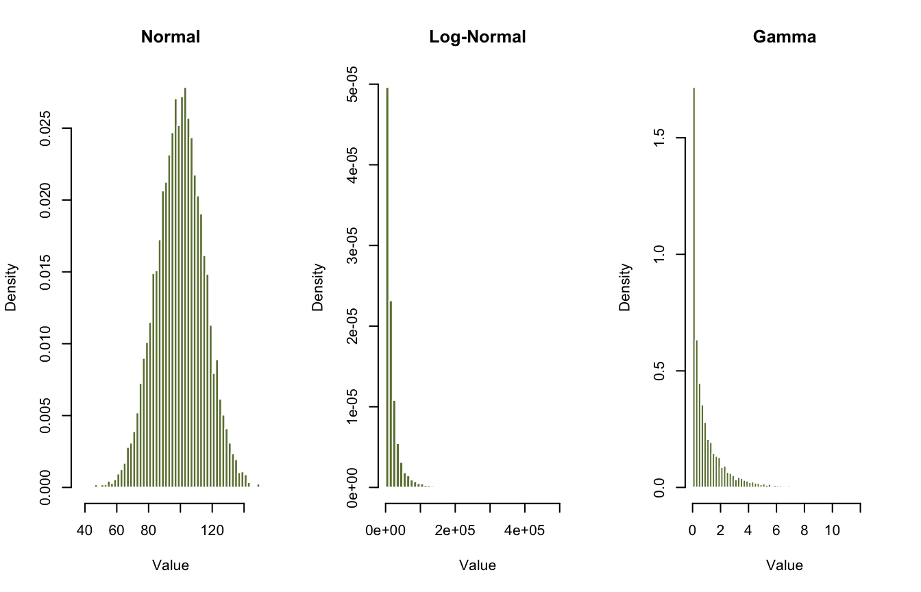

par(op)

sample_skew <- function(x) {
  # Adjusted Fisher-Pearson sample skewness (same formula as the Python twin).
  n <- length(x)
  g1 <- mean((x - mean(x))^3) / mean((x - mean(x))^2)^1.5
  g1 * sqrt(n * (n - 1)) / (n - 2)
}

stats_df <- data.frame(
  Distribution = c("Normal", "Log-Normal", "Gamma"),
  Sample.Mean = c(mean(normal_samples), mean(lognormal_samples),
                  mean(gamma_samples)),
  Sample.Std = c(sd(normal_samples), sd(lognormal_samples),
                 sd(gamma_samples)),
  Sample.Skew = c(sample_skew(normal_samples), sample_skew(lognormal_samples),
                  sample_skew(gamma_samples))
)
cat("\nSample statistics (seed=42):\n")


Sample statistics (seed=42):

print(stats_df, row.names = FALSE)

 Distribution  Sample.Mean   Sample.Std Sample.Skew
       Normal 9.990013e+01    14.994543 -0.04476462
   Log-Normal 1.902829e+04 29289.105202  5.59911505
        Gamma 9.875893e-01     1.382078  2.68244489

Latin hypercube sampling

Latin hypercube sampling (LHS) is a stratified sampling technique. Each dimension’s \([0, 1)\) range is divided into \(n\) equal strata and exactly one sample lands in each stratum:

\[ x_{ij} = \frac{\pi_j(i) + U_{ij}}{n}, \quad i = 0, \ldots, n-1 \]

where \(\pi_j\) is an independent random permutation for each dimension and \(U_{ij} \sim \text{Uniform}(0, 1)\). The median = TRUE variant replaces \(U_{ij}\) with 0.5, placing each point at its stratum center. Projected onto any single axis, the samples fall exactly one per stratum, which removes the clustering and gaps of simple random sampling. LHS often reaches the accuracy of plain Monte Carlo with 5 to 10 times fewer samples.

When to use: Monte Carlo with a limited budget, sensitivity analysis, calibration of expensive models, risk assessment.

lhs <- latin_hypercube(200, 2, seed = 12345)

plot(lhs[, 1], lhs[, 2], pch = 16, cex = 0.6, col = slate,
     main = "Latin hypercube samples (Uniform [0,1])",
     xlab = "Dim 1", ylab = "Dim 2")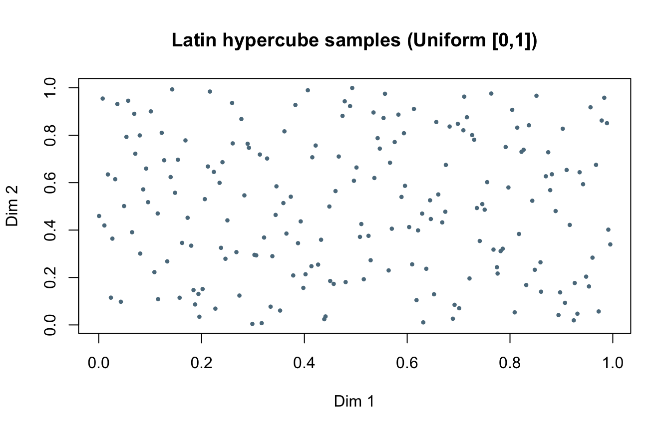

# The defining property: sorted samples in each dimension fall one per stratum.
n <- nrow(lhs)
stratified <- all(vapply(seq_len(ncol(lhs)), function(j) {
  s <- sort(lhs[, j])
  all(s >= (seq_len(n) - 1) / n & s < seq_len(n) / n)
}, logical(1)))
cat("One sample per stratum in every dimension:", stratified, "\n")

One sample per stratum in every dimension: TRUE

Comparing multiple distributions

More than one distribution may fit a dataset well, so it pays to consider several candidates. Here we simulate 50 years of annual peak flows from a Log-Normal distribution (seeded, so the data reproduce exactly) and fit three candidates by maximum likelihood. Every family fits through dist_fit(); GEV also has a dedicated gev_fit() helper whose bespoke path carries quantile standard errors. Distribution fitting is covered properly in the next example.

# Simulate flood frequency data (seeded; upstream uses the same seed)
observed_data <- dist_random(distribution("LogNormal", c(8, 0.6)),
                             50, seed = 123)

lognormal_fit <- dist_fit("LogNormal", observed_data, method = "mle")
weibull_fit <- dist_fit("Weibull", observed_data, method = "mle")
gev_fitted <- dist_fit("GeneralizedExtremeValue", observed_data, method = "mle")
g <- dist_params(gev_fitted)

print(lognormal_fit)

<corehydro_dist> LogNormal(µ = 8.01748, σ = 0.383659)

cat("Weibull fit: params =", round(dist_params(weibull_fit), 4), "\n")

Weibull fit: params = 162478206 1.0237

cat("GEV fit:\n")

GEV fit:

print(g)

            ξ             α             κ 
 8.061729e+07  6.246972e+07 -3.892413e-01

hist(observed_data, breaks = 20, freq = FALSE, col = gray, border = "white",
     main = "Comparing distribution fits", xlab = "Annual peak flow",
     ylab = "Density")
x <- seq(min(observed_data), max(observed_data), length.out = 500)
lines(x, dist_pdf(lognormal_fit, x), col = olive, lwd = 2)
lines(x, dist_pdf(gev_fitted, x), col = clay, lwd = 2)
lines(x, dist_pdf(weibull_fit, x), col = slate, lwd = 2)
legend("topright",
       legend = c("Observed data", "Log-Normal", "GEV", "Weibull"),
       col = c(gray, olive, clay, slate), lwd = c(8, 2, 2, 2), bty = "n")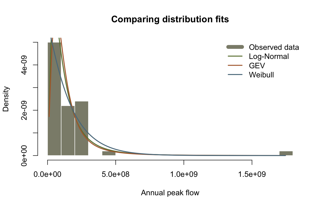

Distribution selection guide

Distribution	Type	Typical use case	Parameters
Normal	Continuous	Symmetric data, measurements	\(\mu\), \(\sigma\)
Log-Normal	Continuous	Right-skewed positive data	\(\mu\), \(\sigma\)
Uniform	Continuous	Equal probability over range	min, max
Triangular	Continuous	Bounded with mode	min, mode, max
PERT	Continuous	Project estimates	min, mode, max
Gamma	Continuous	Positive data, waiting times	\(\theta\), \(\kappa\)
Weibull	Continuous	Reliability, failure time	\(\lambda\), \(\kappa\)
Exponential	Continuous	Time between events	\(\lambda\)
Gumbel	Continuous	Extreme maxima	\(\xi\), \(\alpha\)
GEV	Continuous	General extreme values	\(\xi\), \(\alpha\), \(\kappa\)
Beta	Continuous	Proportions on [0,1]	\(\alpha\), \(\beta\)
Poisson	Discrete	Count data, rare events	\(\lambda\)
Binomial	Discrete	Binary outcomes, trials	\(n\), \(p\)
Bernoulli	Discrete	Single trial success/failure	\(p\)

Summary

You have now explored:

Creating distributions with different parameters.
Computing PDF, CDF, and quantile values.
Generating random samples, including Latin hypercube designs.
Visualizing distributions.
Understanding when to use each distribution.

Exercise

Try creating and plotting these distributions on your own (use dist_params(d) to check the constructor order):

distribution("Beta", c(2, 5)) - useful for probabilities and proportions.
distribution("StudentT", ...) with 3 degrees of freedom - a heavy-tailed alternative to the Normal.
distribution("ChiSquared", c(5)) - goodness-of-fit testing.

Reproduction check

Values printed by the upstream notebook (run against the real C# library), compared with this port. Everything here is deterministic, so the match is exact; most upstream tables print 4 decimal places (or 7 significant figures for the Log-Normal), so those rows are compared at the precision upstream shows. The seeded draws, the Latin hypercube design, and the fitted parameters are additionally asserted bit-identical to the Python version of this page.

Quantity	Upstream C#	This port	Status
`Normal(100,15).InverseCDF(0.05)`	75.32719559572791	`dist_quantile(normal, 0.05)`	exact
`Normal(100,15).InverseCDF(0.95)`	124.67280440427207	`dist_quantile(normal, 0.95)`	exact
`LogNormal(4,0.5).Mean`	1.940096e+04	`dist_moments()[["mean"]]`	exact (7 sig figs shown)
`LogNormal(4,0.5).Kurtosis`	346.8718	`dist_moments()[["kurtosis"]]`	exact (4 dp shown)
`LogNormal(4,0.5).InverseCDF(0.95)`	6.643957e+04	`dist_quantile(., 0.95)`	exact (7 sig figs shown)
GEV(100,15,-0.5) mean / min	123.1736 / 70.0	`dist_moments()`	exact (4 dp shown)
GEV(100,15,0) mean / sd	108.6582 / 19.2382	`dist_moments()`	exact (4 dp shown)
GEV(100,15,0.5) mean / max	103.4132 / 130.0	`dist_moments()`	exact (4 dp shown)
Gamma(2,0.5) mean / kurtosis	1.0 / 15.0	`dist_moments()`	exact
Gamma(2,0.5).InverseCDF(0.95)	3.8415	`dist_quantile(., 0.95)`	exact (4 dp shown)
Weibull(100,2.5) mean	88.7264	`dist_moments()[["mean"]]`	exact (4 dp shown)
Uniform(0,100) sd / kurtosis	28.8675 / 1.8	`dist_moments()`	exact
Triangular(0,30,100) mean / median	43.3333 / 40.8392	`dist_moments()`, `dist_quantile()`	exact (4 dp shown)
PERT(10,50,100) mean / median	51.6667 / 51.2732	`dist_moments()`, `dist_quantile()`	exact (4 dp shown)
Poisson(3.5) P(X=3) / P(X<=5)	0.2158 / 0.8576	`dist_pdf(., 3)`, `dist_cdf(., 5)`	exact (4 dp shown)
Binomial(0.3,20) mean / 95th pct	6.0 / 9.0	`dist_moments()`, `dist_quantile()`	exact
First draw, `LogNormal(8,0.6)` seed 123	(not printed upstream)	bit-identical to Python twin	exact
LHS(200, 2, seed 12345) first point	(not printed upstream)	bit-identical to Python twin	exact

The chunk below fails the render if any value drifts. The final block asserts the cross-language guarantee: the seeded draws, the Latin hypercube design, and the fitted Log-Normal parameters are the exact values the Python notebook prints.

# Upstream reference values: 01_distributions.ipynb, cells 4, 8, 10, 12, 14,
# 16, 18, 20, 22, 24 outputs. Upstream tables print DataFrame.round(4), so
# 4-decimal literals are compared at that precision; the underlying math is
# deterministic.
shown <- function(x, literal, tol = 5e-5) abs(x - literal) < tol

# Long-decimal literals are compared with a 1e-15 relative tolerance only
# because R's decimal parser can land one ulp away from the written literal.
rel <- function(x, literal, tol = 1e-15) abs(x / literal - 1) < tol

# Normal(100, 15) -- full-precision prints upstream
stopifnot(
  rel(dist_quantile(normal, 0.05), 75.32719559572791),
  dist_quantile(normal, 0.5) == 100.0,
  rel(dist_quantile(normal, 0.95), 124.67280440427207)
)

# LogNormal(4, 0.5) -- shown to 7 significant figures upstream
ln_m <- dist_moments(lognormal)
stopifnot(
  rel(ln_m[["mean"]], 1.940096e4, tol = 1e-6),
  rel(ln_m[["sd"]], 3.225447e4, tol = 1e-6),
  shown(ln_m[["skewness"]], 9.5827),
  shown(ln_m[["kurtosis"]], 346.8718),
  rel(dist_quantile(lognormal, 0.05), 1.505127e3, tol = 1e-6),
  rel(dist_quantile(lognormal, 0.95), 6.643957e4, tol = 1e-6)
)

# GEV shapes
fm <- dist_moments(gev_frechet)
gm <- dist_moments(gev_gumbel)
wm <- dist_moments(gev_weibull)
stopifnot(
  shown(fm[["mean"]], 123.1736), fm[["minimum"]] == 70.0,
  shown(dist_quantile(gev_frechet, 0.95), 202.4619),
  shown(gm[["mean"]], 108.6582), shown(gm[["sd"]], 19.2382),
  shown(gm[["skewness"]], 1.1396), gm[["kurtosis"]] == 5.4,
  shown(dist_quantile(gev_gumbel, 0.5), 105.4977),
  shown(wm[["mean"]], 103.4132), wm[["maximum"]] == 130.0,
  shown(dist_quantile(gev_weibull, 0.95), 123.2056)
)

# Gamma(2, 0.5)
gam_m <- dist_moments(gamma_dist)
stopifnot(
  gam_m[["mean"]] == 1.0, gam_m[["kurtosis"]] == 15.0,
  shown(gam_m[["sd"]], 1.4142), shown(gam_m[["skewness"]], 2.8284),
  shown(dist_quantile(gamma_dist, 0.5), 0.4549),
  shown(dist_quantile(gamma_dist, 0.95), 3.8415)
)

# Weibull(100, 2.5)
wb_m <- dist_moments(weibull)
stopifnot(
  shown(wb_m[["mean"]], 88.7264), shown(wb_m[["sd"]], 37.9667),
  shown(dist_quantile(weibull, 0.95), 155.0962)
)

# Uniform, Triangular, PERT
un_m <- dist_moments(uniform)
tr_m <- dist_moments(triangular)
pt_m <- dist_moments(pert)
stopifnot(
  un_m[["mean"]] == 50.0, un_m[["kurtosis"]] == 1.8,
  shown(un_m[["sd"]], 28.8675),
  shown(tr_m[["mean"]], 43.3333), shown(tr_m[["skewness"]], 0.3561),
  shown(dist_quantile(triangular, 0.5), 40.8392),
  shown(dist_quantile(triangular, 0.95), 81.2917),
  shown(pt_m[["mean"]], 51.6667), shown(pt_m[["sd"]], 16.9617),
  shown(dist_quantile(pert, 0.5), 51.2732),
  shown(dist_quantile(pert, 0.95), 80.2234)
)

# Poisson(3.5) and Binomial(0.3, 20)
po_m <- dist_moments(poisson)
bi_m <- dist_moments(binomial)
stopifnot(
  po_m[["mean"]] == 3.5, shown(po_m[["sd"]], 1.8708),
  shown(dist_pdf(poisson, 3), 0.2158),
  shown(dist_cdf(poisson, 5), 0.8576),
  dist_quantile(poisson, 0.95) == 7.0,
  bi_m[["mean"]] == 6.0, shown(bi_m[["sd"]], 2.0494),
  dist_quantile(binomial, 0.05) == 3.0,
  dist_quantile(binomial, 0.95) == 9.0
)

# Seeded values, bit-identical across R, Python, and the C# library
stopifnot(
  rel(normal_samples[1], 95.20221411105254),
  rel(observed_data[1], 203499515.64666739),
  rel(lhs[1, 1], 0.12249509909539484),
  rel(lhs[1, 2], 0.81019698383868677),
  stratified
)
# Log-Normal MLE is deterministic (closed-form in log space); the tolerance
# only guards platform libm differences.
ln_params <- dist_params(lognormal_fit)
stopifnot(
  rel(ln_params[[1]], 8.0174794125819, tol = 1e-12),
  rel(ln_params[[2]], 0.383659272555292, tol = 1e-12)
)

cat("All reproduction checks passed.\n")

All reproduction checks passed.