22. Reliability analysis

Language: R (Quarto) - Python version

Ported from reliability_analysis.py in the USACE-RMC Numerics-Python-Examples repository (0BSD licensed). The upstream script drives the C# Numerics.dll through pythonnet; this version uses corehydror, whose compiled core is a validated C++ port of the same library. The Python version of this example uses the same core and prints the same numbers.

This example runs a Monte Carlo reliability analysis of the classic resistance-minus-load limit state. A component fails when the load S it carries exceeds the resistance R it can supply, so the limit-state function is g = R - S and failure is the event g <= 0. Simulating both random variables many times estimates the failure probability Pf directly, and the reliability index beta = -Φ^-1(Pf) restates that probability on a standard-normal scale.

What you’ll learn

• How to model a log-normal resistance and a Normal load with corehydror.
• How to estimate a failure probability and reliability index by Monte Carlo simulation.
• How the port’s LnNormal family replaces the upstream base-e LogNormal workaround.

Setup

The upstream script spends about forty lines resolving Numerics.dll from the NuGet cache and loading the CoreCLR runtime before it can start. None of that exists here.

library(corehydror)

Define the random variables

Resistance R is log-normal with a physical-space mean of 500 and standard deviation of 120. Load S is Normal with mean 380 and standard deviation 90.

The upstream script has to work for its log-normal: the C# LogNormal class is base-10 and takes log-space parameters, so the script converts the physical mean and standard deviation to (mu_ln, sigma_ln) by hand and then mutates resistance_dist.Base = e. That .Base mutation is not exposed by this port. Instead the port ships LnNormal, the library’s base-e log-normal family, and LnNormal is parameterized in real space: you pass the physical mean and standard deviation directly, and the class performs the same moment conversion internally (its DirectMethodOfMoments is exactly the algebra the upstream script writes out). The whole construction collapses to one line.

To show the two parameterizations agree, the chunk below repeats the upstream hand conversion and checks it against the fitted family: a log-normal’s median is exp(mu_ln), and the physical moments round-trip.

resistance_mean <- 500
resistance_std <- 120
resistance_dist <- distribution("LnNormal", c(resistance_mean, resistance_std))
load_dist <- distribution("Normal", c(380, 90))

# The upstream hand conversion, kept only as a cross-check
sigma2_ln <- log1p((resistance_std / resistance_mean)^2)
mu_ln <- log(resistance_mean) - 0.5 * sigma2_ln
cat(sprintf("hand-converted mu_ln = %.6f, sigma_ln = %.6f\n", mu_ln, sqrt(sigma2_ln)))

hand-converted mu_ln = 6.186607, sigma_ln = 0.236648

cat(sprintf("exp(mu_ln)      = %.10f\n", exp(mu_ln)))

exp(mu_ln)      = 486.1936509903

cat(sprintf("LnNormal median = %.10f\n", dist_quantile(resistance_dist, 0.5)))

LnNormal median = 486.1936509903

m <- dist_moments(resistance_dist)
cat(sprintf(
  "LnNormal mean = %.6f, sd = %.6f  (round-trips to 500, 120)\n",
  m[["mean"]], m[["sd"]]
))

LnNormal mean = 500.000000, sd = 120.000000  (round-trips to 500, 120)

Monte Carlo simulation

Draw 100,000 samples of each variable with the upstream seeds (42 for resistance, 43 for load). The port keeps the C# Mersenne Twister bit-exact, so the streams below are the same numbers the upstream script draws from Numerics.dll, and the Python twin draws them identically.

n_samples <- 100000
r <- dist_random(resistance_dist, n_samples, seed = 42)
s <- dist_random(load_dist, n_samples, seed = 43)
g <- r - s

Failure probability and reliability index

Pf is the fraction of samples with g <= 0, and beta = -Φ^-1(Pf). The upstream script computes beta with scipy.stats.norm.ppf; here qnorm supplies the same function, and the Python twin uses the port’s own standard Normal inverse CDF and prints the identical value.

n_fail <- sum(g <= 0)
pf <- mean(g <= 0)
beta <- -qnorm(pf)

summary_df <- data.frame(
  Metric = c(
    "Samples", "Failures", "Mean resistance", "Std resistance",
    "Mean load", "Std load", "Pf", "beta"
  ),
  Value = round(c(n_samples, n_fail, mean(r), sd(r), mean(s), sd(s), pf, beta), 6)
)
cat("Reliability analysis summary:\n")

Reliability analysis summary:

print(summary_df, row.names = FALSE)

          Metric        Value
         Samples 100000.00000
        Failures  21423.00000
 Mean resistance    499.86000
  Std resistance    119.78269
       Mean load    380.32862
        Std load     89.90154
              Pf      0.21423
            beta      0.79183

The first ten simulated samples, as the upstream script prints them:

sample_df <- data.frame(
  Resistance = r[1:10], Load = s[1:10], "g = R - S" = g[1:10],
  check.names = FALSE
)
cat("First 10 simulated samples:\n")

First 10 simulated samples:

print(round(sample_df, 3), row.names = FALSE)

 Resistance    Load g = R - S
    450.751 271.993   178.758
    591.622 379.292   212.330
    718.745 404.920   313.825
    392.708 266.140   126.569
    562.875 280.055   282.820
    583.531 286.246   297.285
    515.811 316.603   199.207
    515.240 294.881   220.360
    382.744 339.696    43.048
    470.773 459.355    11.418

Plots

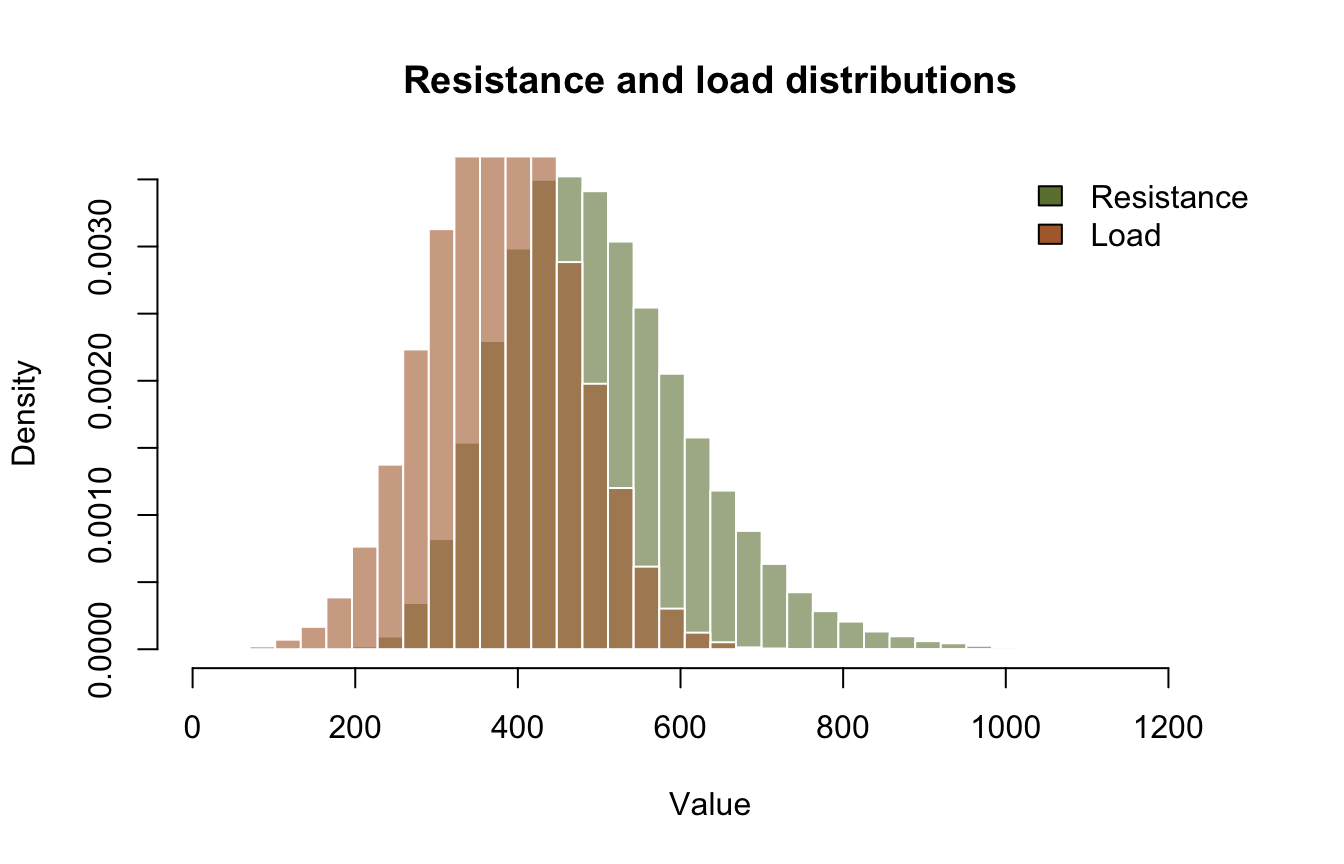
The upstream script draws one 2x2 figure; here the same four panels are drawn as separate figures at the site’s default size. First, the two input distributions overlaid:

brks <- seq(min(r, s), max(r, s), length.out = 41)
hist(r,
  breaks = brks, freq = FALSE, col = adjustcolor("#6b7f3f", 0.6),
  border = "white", main = "Resistance and load distributions",
  xlab = "Value", ylab = "Density"
)
hist(s,
  breaks = brks, freq = FALSE, col = adjustcolor("#b06a3b", 0.6),
  border = "white", add = TRUE
)
legend("topright",
  legend = c("Resistance", "Load"),
  fill = c("#6b7f3f", "#b06a3b"), bty = "n"
)

The limit-state distribution. Everything left of the dashed line is a failure:

hist(g,
  breaks = 50, col = "#5b7a8c", border = "white",
  main = "Limit-state distribution", xlab = "g = R - S"
)
abline(v = 0, col = "#b06a3b", lty = 2, lwd = 2)
legend("topright", legend = "Failure boundary g = 0", col = "#b06a3b", lty = 2, bty = "n")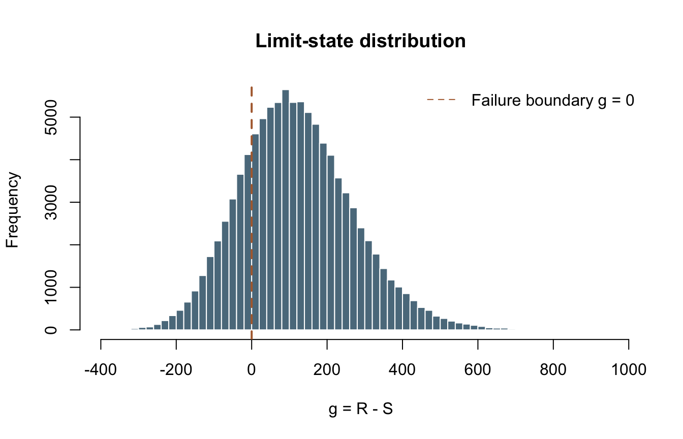

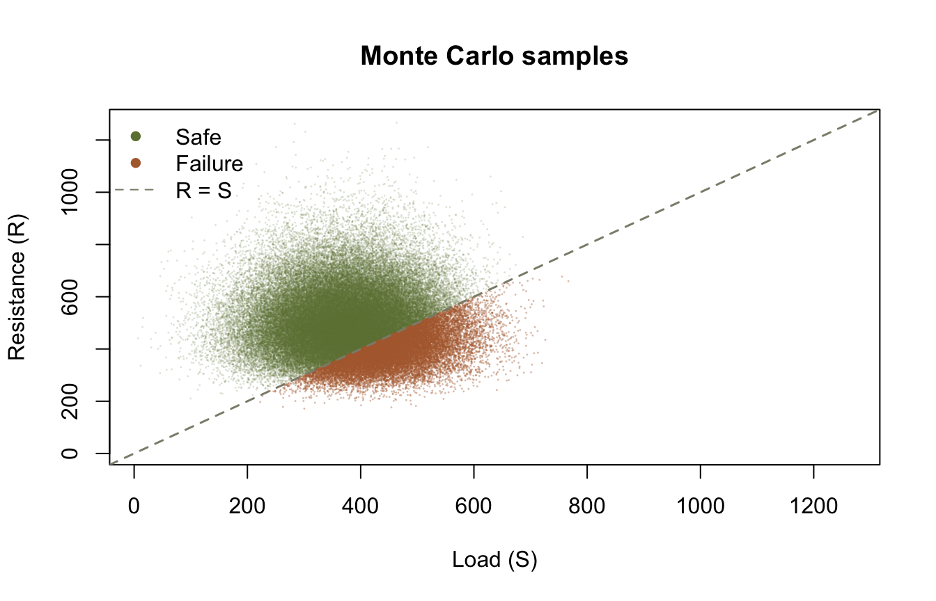
The samples in (load, resistance) space. Failures are the points below the R = S line:

fail <- g <= 0
plot(s[!fail], r[!fail],
  pch = 16, cex = 0.2, col = adjustcolor("#6b7f3f", 0.2),
  xlim = range(s, r), ylim = range(s, r),
  xlab = "Load (S)", ylab = "Resistance (R)", main = "Monte Carlo samples"
)
points(s[fail], r[fail], pch = 16, cex = 0.2, col = adjustcolor("#b06a3b", 0.4))
abline(0, 1, lty = 2, lwd = 1.5, col = "#8c8c7a")
legend("topleft",
  legend = c("Safe", "Failure", "R = S"),
  col = c("#6b7f3f", "#b06a3b", "#8c8c7a"),
  pch = c(16, 16, NA), lty = c(NA, NA, 2), bty = "n"
)

And the empirical CDF of g. Its value at the dashed line is Pf:

plot(sort(g), seq_along(g) / length(g),
  type = "l", lwd = 2, col = "#5b7a8c",
  xlab = "g = R - S", ylab = "Empirical CDF",
  main = "Empirical CDF of the limit state"
)
abline(v = 0, col = "#b06a3b", lty = 2, lwd = 2)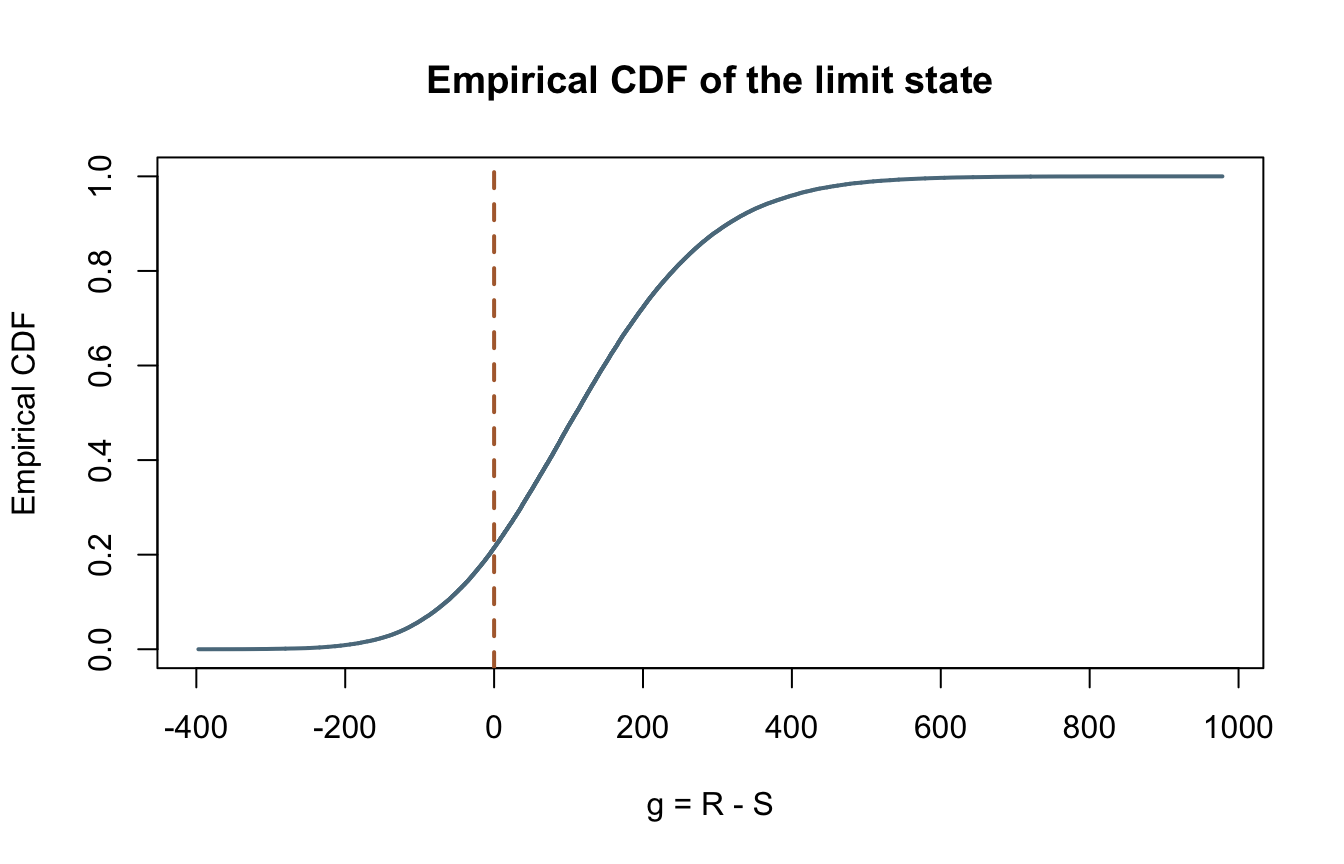

Reproduction check

The upstream file is a standalone script that prints its results at runtime; the repository does not embed them, so there are no upstream literals to pin against. The check below therefore asserts two things, stated plainly: internal consistency (the LnNormal physical moments round-trip and the upstream hand conversion reproduces the internal one), and cross-language identity (the Python twin asserts exactly the same literals, which only pass because the seeded draws, Pf, and beta are fully deterministic and bit-identical in both languages).

Quantity	Upstream C#	This port	Status
First resistance draw (seed 42)	not embedded upstream	450.7507979426037	exact (cross-language)
First load draw (seed 43)	not embedded upstream	271.992998170271	exact (cross-language)
First limit-state value g	not embedded upstream	178.7577997723327	exact (cross-language)
Failures out of 100,000	not embedded upstream	21423	exact (cross-language)
Pf	not embedded upstream	0.21423	exact (cross-language)
beta	not embedded upstream	0.7918296694786122	exact (cross-language)
LnNormal(500, 120) mean, sd	500, 120 by construction	m[["mean"]], m[["sd"]]	exact (round trip, 1e-12)

The chunk below fails the render if any value drifts.

# Upstream: examples/reliability_analysis.py (standalone script, prints at runtime,
# no embedded outputs). Cross-language identity with the Python twin is the oracle
# here. The values are bit-exact (the fixture suite enforces the seeded stream);
# the comparisons carry a 1e-15 relative tolerance only because R's decimal parser
# can land one ulp away from the written literal.
stopifnot(
  abs(r[1] / 450.7507979426037 - 1) < 1e-15,
  abs(s[1] / 271.992998170271 - 1) < 1e-15,
  abs(g[1] / 178.7577997723327 - 1) < 1e-15,
  n_fail == 21423,
  pf == 0.21423,
  abs(beta / 0.7918296694786122 - 1) < 1e-15
)
# Internal consistency: LnNormal(500, 120) round-trips its physical moments and
# the upstream hand conversion matches the internal one (median = exp(mu_ln)).
stopifnot(
  abs(m[["mean"]] / 500 - 1) < 1e-12,
  abs(m[["sd"]] / 120 - 1) < 1e-12,
  abs(dist_quantile(resistance_dist, 0.5) / exp(mu_ln) - 1) < 1e-14
)
cat("All reproduction checks passed.\n")

All reproduction checks passed.