05. Adaptive MCMC samplers

Language: R (Quarto) - Python version

Ported from 05_mcmc_adaptive.ipynb in the USACE-RMC Numerics-Python-Examples repository (0BSD licensed). The upstream notebook drives the C# Numerics.dll through pythonnet; this version uses corehydror, whose compiled core is a validated C++ port of the same library. The seeded data and every posterior summary printed below are bit-identical to the Python version of this example, which runs the same core stream. Comparisons against the upstream notebook’s printed posteriors are statistical rather than exact because the priors differ (see the reproduction check at the end).

What you’ll learn

• Why adaptive MCMC improves mixing without manual proposal tuning.
• How ARWMH learns the proposal covariance during warmup.
• How DEMCz and DEMCzs build proposals from a population of past states.
• How HMC and NUTS use gradient information to explore efficiently.
• How to compare samplers using acceptance rate, R-hat, and effective sample size.

Setup

The upstream notebook loads the CoreCLR runtime through pythonnet, resolves Numerics.dll, wraps a log-likelihood function in a .NET LogLikelihood delegate, builds a List[IUnivariateDistribution] of priors, and disables the samplers’ internal chain parallelism to avoid GIL contention. None of that exists here. mcmc_sample() fits a named distribution family to the data and returns the chains, acceptance rates, posterior summaries, and diagnostics in one call.

One honest difference to keep in mind throughout: the upstream notebook hand-picks its priors (Uniform(50, 150) for \(\mu\) and Uniform(5, 30) for \(\sigma\) in the Normal example). corehydror does not expose custom priors; mcmc_sample() always uses uniform priors spanning the family’s parameter constraints, exactly the C# GetParameterConstraints bounds. With data this informative the posteriors are nearly the same, but bit-comparison against the upstream outputs is impossible, so the reproduction check treats every upstream posterior value as a statistical comparison.

library(corehydror)

Adaptive Random Walk Metropolis-Hastings (ARWMH)

We start with the most basic adaptive sampler: Adaptive Random Walk Metropolis-Hastings, which tunes the proposal distribution automatically during warmup [1].

Mathematical foundation

The proposal at iteration \(t\) uses a mixture:

\[ \theta^* \sim \begin{cases} \mathcal{N}\!\left(\theta, \, \frac{0.1^2}{d} \, I_d\right) & \text{with probability } \beta \\ \mathcal{N}\!\left(\theta, \, \frac{2.38^2}{d} \, \hat{\Sigma}_t\right) & \text{with probability } 1-\beta \end{cases} \]

where \(d\) is the number of parameters, \(\beta = 0.05\) by default, \(\hat{\Sigma}_t\) is the running covariance of the chain’s accepted samples, and \(I_d\) is the identity matrix. The small identity component, also used for the first \(100 \times d\) samples, keeps the chain ergodic even when the adaptive covariance estimate is poor. Both proposal components are symmetric, so the acceptance criterion reduces to the plain posterior ratio, exactly as in RWMH.

When to use ARWMH:

• Medium-dimensional problems (2 to 20 parameters).
• Correlated parameters.
• When you do not want to tune proposals by hand. It is a sound default for most applications.

We generate 100 seeded draws from a Normal(100, 15), then recover the parameters. The seed reproduces the C# Mersenne Twister stream bit-for-bit, so data matches the upstream notebook’s synthetic data and the Python twin exactly.

true_mu <- 100
true_sigma <- 15
data <- dist_random(distribution("Normal", c(true_mu, true_sigma)), 100, seed = 1234)
cat(sprintf("first draw: %.14f, sample mean: %.3f\n", data[1], mean(data)))

first draw: 86.91533945543637, sample mean: 100.615

arwmh <- mcmc_sample(
  data, distribution = "Normal", sampler = "ARWMH",
  iterations = 2500, warmup = 800, chains = 4, thinning = 1, seed = 12345
)

summary_df <- data.frame(
  parameter = arwmh$parameters,
  true = c(true_mu, true_sigma),
  posterior_mean = arwmh$posterior_mean,
  posterior_sd = arwmh$posterior_sd,
  rhat = arwmh$rhat,
  ess = arwmh$ess
)
cat("ARWMH results\n")

ARWMH results

print(summary_df, row.names = FALSE, digits = 5)

 parameter true posterior_mean posterior_sd   rhat    ess
         µ  100        100.657       1.5233 1.0003 1222.2
         σ   15         15.097       1.1275 1.0035 1158.5

cat("\nacceptance rate by chain:", round(arwmh$acceptance_rates, 3), "\n")

acceptance rate by chain: 0.405 0.436 0.444 0.441 

The acceptance rates sit near the 0.3 to 0.4 range that is close to optimal for random-walk samplers in low dimensions, with no manual tuning. Trace plots confirm the chains mix well around the posterior mean:

mu_draws <- unlist(lapply(arwmh$chains, function(c) c[, 1]))
sigma_draws <- unlist(lapply(arwmh$chains, function(c) c[, 2]))

op <- par(mfrow = c(2, 1), mar = c(4, 4, 2, 1))
plot(mu_draws, type = "l", lwd = 0.4, col = "#5b7a8c",
     xlab = "", ylab = "mu", main = "ARWMH trace, Normal fit")
abline(h = mean(mu_draws), col = "#b06a3b", lty = 2, lwd = 1.5)
plot(sigma_draws, type = "l", lwd = 0.4, col = "#5b7a8c",
     xlab = "draw (chains concatenated)", ylab = "sigma")
abline(h = mean(sigma_draws), col = "#b06a3b", lty = 2, lwd = 1.5)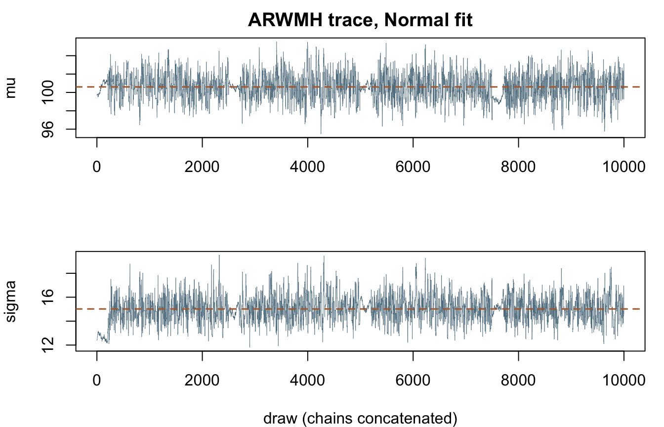

par(op)

Differential Evolution MCMC (DEMCz and DEMCzs)

Differential Evolution MCMC (DEMCz) is a population-based sampler [2]. DEMCz with snooker update (DEMCzs) is an enhanced version with better mixing.

Mathematical foundation

DEMCz generates proposals from the difference of two past states drawn from a population matrix \(Z\), a memory of past states from all chains:

\[ \theta^*_i = \theta_i + \gamma \, (z_{R_1} - z_{R_2}) + e \]

where \(\gamma = 2.38 / \sqrt{2d}\) is the default jump rate, \(z_{R_1}\) and \(z_{R_2}\) are two randomly selected past states, and \(e \sim \mathcal{N}(0, b^2)\) is a small noise perturbation with \(b = 10^{-3}\). With probability 0.1 the jump rate is set to \(\gamma = 1\), which jumps the full difference between two past states and lets the chain bridge separated modes. The population matrix learns the scale and orientation of the posterior on its own, so no proposal covariance needs to be specified. The snooker update in DEMCzs adds proposals along the line through the current state and a random past state, which further improves mixing in awkward geometries.

When to use DEMCz or DEMCzs:

• High-dimensional problems (20+ parameters).
• Multimodal posteriors or complex posterior geometry.
• When ARWMH struggles with convergence.

The upstream notebook’s advice holds here too: DEMCzs is the fastest and most robust of these samplers, and the best adaptive method to default to. It is also the default sampler used by the *_analysis functions elsewhere in this package.

demczs_norm <- mcmc_sample(
  data, distribution = "Normal", sampler = "DEMCzs",
  iterations = 2500, warmup = 800, chains = 4, thinning = 1, seed = 12345
)

summary_df <- data.frame(
  parameter = demczs_norm$parameters,
  true = c(true_mu, true_sigma),
  posterior_mean = demczs_norm$posterior_mean,
  posterior_sd = demczs_norm$posterior_sd,
  rhat = demczs_norm$rhat,
  ess = demczs_norm$ess
)
cat("DEMCzs results\n")

DEMCzs results

print(summary_df, row.names = FALSE, digits = 5)

 parameter true posterior_mean posterior_sd   rhat    ess
         µ  100        100.644       1.5236 1.0004 1219.6
         σ   15         14.997       1.0647 1.0051 1128.5

cat("\nacceptance rate by chain:", round(demczs_norm$acceptance_rates, 3), "\n")

acceptance rate by chain: 0.369 0.354 0.36 0.362 

Comparing MCMC samplers

Different samplers have different strengths. We compare all five adaptive samplers the port exposes (plain RWMH and SNIS are also available through the same interface):

• ARWMH: adaptive random walk (auto-tuned covariance).
• DEMCz: differential evolution (population-based proposals).
• DEMCzs: DEMCz with snooker update (better mixing).
• HMC: Hamiltonian Monte Carlo (gradient-based).
• NUTS: No-U-Turn Sampler (adaptive HMC).

HMC mathematical foundation

Hamiltonian Monte Carlo augments the parameter space with momentum variables \(\phi\) and simulates Hamiltonian dynamics to generate distant, high-quality proposals [3][4]:

\[ H(\theta, \phi) = U(\theta) + K(\phi) = -\log \pi(\theta) + \frac{1}{2} \phi^T M^{-1} \phi \]

where \(U(\theta)\) is the potential energy (negative log-posterior), \(K(\phi)\) is the kinetic energy, and the mass matrix \(M\) is diagonal in this implementation. HMC is very efficient on smooth posteriors (low autocorrelation, fast exploration) but needs gradients, is less robust to discontinuities, and its trajectory length must be tuned by hand.

NUTS mathematical foundation

The No-U-Turn Sampler removes HMC’s most sensitive tuning parameter, the number of leapfrog steps, by growing the trajectory until it starts to double back on itself [5]. It builds a balanced binary tree of leapfrog states and stops when the U-turn criterion triggers:

\[ (\theta^+ - \theta^-) \cdot \phi^- < 0 \quad \text{or} \quad (\theta^+ - \theta^-) \cdot \phi^+ < 0 \]

where \(\theta^{\pm}\) are the trajectory endpoints and \(\phi^{\pm}\) their momenta. Step size is adapted automatically by dual averaging, which makes NUTS the recommended gradient-based sampler for most problems.

A compact guide:

Sampler	Best for	Notes
ARWMH	2-20 parameters, correlated parameters	Sound default, no tuning
DEMCz	High dimensions, multimodal posteriors	Population supplies the proposal scale
DEMCzs	Same as DEMCz	Fastest and most robust; default to this
HMC	Smooth, differentiable posteriors	Needs step size and step count tuning
NUTS	Smooth posteriors, no tuning appetite	Self-tuning HMC, costlier per draw

Gumbel example

We fit a Gumbel distribution to seeded synthetic data with all five samplers. The Gumbel is a good test case for the gradient-based samplers because its log-density is smooth and cheap to differentiate numerically, so HMC and NUTS avoid the step-size thrashing that heavier-tailed families can induce. HMC and NUTS get smaller iteration budgets because each of their iterations costs many gradient evaluations.

true_xi <- 10.0    # location
true_alpha <- 2.0  # scale
gumbel_data <- dist_random(distribution("Gumbel", c(true_xi, true_alpha)), 50, seed = 12345)
cat(sprintf("first draw: %.15f, sample mean: %.3f\n", gumbel_data[1], mean(gumbel_data)))

first draw: 15.235041366837393, sample mean: 11.630

settings <- list(
  ARWMH  = list(iterations = 2500, warmup = 800, chains = 4),
  DEMCz  = list(iterations = 2500, warmup = 800, chains = 4),
  DEMCzs = list(iterations = 2500, warmup = 800, chains = 4),
  HMC    = list(iterations = 2000, warmup = 600, chains = 2),
  NUTS   = list(iterations = 1200, warmup = 400, chains = 2)
)

runs <- list()
rows <- list()
for (name in names(settings)) {
  cfg <- settings[[name]]
  t0 <- Sys.time()
  r <- mcmc_sample(
    gumbel_data, distribution = "Gumbel", sampler = name,
    iterations = cfg$iterations, warmup = cfg$warmup, chains = cfg$chains,
    thinning = 1, seed = 12345
  )
  elapsed <- as.numeric(difftime(Sys.time(), t0, units = "secs"))
  runs[[name]] <- r
  rows[[name]] <- data.frame(
    sampler = name,
    runtime_s = round(elapsed, 2),
    xi_mean = r$posterior_mean[1],
    alpha_mean = r$posterior_mean[2],
    xi_error = r$posterior_mean[1] - true_xi,
    alpha_error = r$posterior_mean[2] - true_alpha,
    accept = mean(r$acceptance_rates),
    max_rhat = max(r$rhat),
    min_ess = min(r$ess)
  )
}

comparison <- do.call(rbind, rows)
cat("Sampler comparison\n")

Sampler comparison

print(comparison, row.names = FALSE, digits = 4)

 sampler runtime_s xi_mean alpha_mean xi_error alpha_error accept max_rhat
   ARWMH      0.04   10.40      2.370   0.3997      0.3697 0.4035    1.001
   DEMCz      0.02   10.39      2.358   0.3930      0.3581 0.3474    1.001
  DEMCzs      0.02   10.40      2.351   0.3965      0.3508 0.3498    1.003
     HMC      2.36   10.39      2.357   0.3901      0.3574 0.9785    1.000
    NUTS      0.34   10.39      2.350   0.3875      0.3496 1.0000    1.004
 min_ess
    1198
    1226
    1224
    6001
    2846

All five samplers agree on the posterior to two decimal places, matching the upstream notebook’s picture: the random-walk and population samplers finish in milliseconds, while the gradient-based samplers pay for numerical differentiation on every leapfrog step but return chains with very low autocorrelation (note the ESS relative to the number of draws). The posterior from DEMCzs:

best <- runs[["DEMCzs"]]
xi_draws <- unlist(lapply(best$chains, function(c) c[, 1]))
alpha_draws <- unlist(lapply(best$chains, function(c) c[, 2]))

op <- par(mfrow = c(1, 2), mar = c(4, 4, 3, 1))
hist(xi_draws, breaks = 40, freq = FALSE, col = "#6b7f3f", border = "white",
     xlab = "xi (location)", main = "DEMCzs posterior: xi")
abline(v = true_xi, col = "#b06a3b", lty = 2, lwd = 1.5)
hist(alpha_draws, breaks = 40, freq = FALSE, col = "#6b7f3f", border = "white",
     xlab = "alpha (scale)", main = "DEMCzs posterior: alpha")
abline(v = true_alpha, col = "#b06a3b", lty = 2, lwd = 1.5)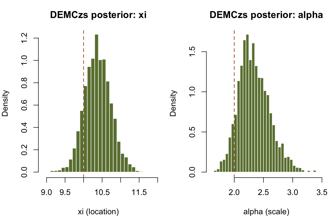

par(op)

What was not ported

The upstream notebook ends with two performance benchmarks against PyMC’s NUTS sampler. Those sections depend on a separate probabilistic-programming stack and compare pythonnet call overhead rather than the library itself, so they are not ported here.

Summary

In this notebook you:

• Used ARWMH to adapt the proposal covariance automatically.
• Applied DEMCz and DEMCzs, whose population of past states supplies the proposal scale.
• Compared the adaptive samplers with the gradient-based HMC and NUTS.
• Read acceptance rates, R-hat, and ESS to judge sampler behavior.

Exercises

1. Run ARWMH and DEMCz on the same problem and compare ESS.
2. Increase the sample size or switch families and note how the samplers respond.
3. Compare NUTS and HMC on a smooth posterior and report acceptance rates.

References

[1] H. Haario, E. Saksman, and J. Tamminen, “An adaptive Metropolis algorithm,” Bernoulli, vol. 7, no. 2, pp. 223-242, 2001.

[2] C. J. F. ter Braak and J. A. Vrugt, “Differential evolution Markov chain with snooker updater and fewer chains,” Statistics and Computing, vol. 18, no. 4, pp. 435-446, 2008.

[3] R. M. Neal, “MCMC using Hamiltonian dynamics,” in Handbook of Markov Chain Monte Carlo. CRC Press, 2011.

[4] M. Betancourt, “A conceptual introduction to Hamiltonian Monte Carlo,” arXiv preprint arXiv:1701.02434, 2017.

[5] M. D. Hoffman and A. Gelman, “The No-U-Turn Sampler: Adaptively setting path lengths in Hamiltonian Monte Carlo,” Journal of Machine Learning Research, vol. 15, no. 47, pp. 1593-1623, 2014.

Reproduction check

The seeded data draws are exact: the port reproduces the C# Mersenne Twister stream bit-for-bit, and the Python twin prints the same values. Every posterior comparison against the upstream notebook is statistical, for two reasons stated honestly: the upstream hand-picks its priors (Uniform(50, 150) and Uniform(5, 30) for the Normal; Uniform(0, 20) and Uniform(0.5, 10) for the Gumbel) while this port always uses the family’s constraint-based uniform priors, and the chain settings differ, so the sampler streams cannot be bit-compared. Two posterior-mean literals are additionally asserted as exact cross-language checks: the Python twin computes the identical values from the same core stream.

Quantity	Upstream C#	This port	Status
ARWMH Normal posterior mean of mu	100.611	~100.657	statistical
ARWMH Normal posterior mean of sigma	15.053	~15.097	statistical
DEMCzs Normal posterior mean of mu	100.596	~100.644	statistical
DEMCzs Normal posterior mean of sigma	15.037	~14.997	statistical
Gumbel xi posterior mean, all 5 samplers	10.375 to 10.422	10.387 to 10.400	statistical
Gumbel alpha posterior mean, all 5 samplers	2.335 to 2.358	2.350 to 2.370	statistical
Seeded Normal / Gumbel data draws	(not printed upstream)	bit-exact vs C# stream and Python twin	exact
ARWMH Normal and DEMCzs Gumbel posterior means	(cross-language identity)	identical in the Python twin	exact

The chunk below fails the render if any check drifts.

# Upstream: 05_mcmc_adaptive.ipynb, cell 7 (ARWMH Normal), cell 9 (DEMCzs Normal),
# cell 12 (Gumbel sampler-comparison table).

# exact: seeded data and cross-language posterior means, identical in the Python
# twin. The values themselves are bit-exact (the fixture suite enforces that); the
# comparisons carry a 1e-15 relative tolerance only because R's decimal parser can
# land one ulp away from the written literal.
stopifnot(
  abs(data[1] / 86.91533945543637 - 1) < 1e-15,
  abs(gumbel_data[1] / 15.235041366837393 - 1) < 1e-15,
  abs(arwmh$posterior_mean[1] / 100.6571453618418 - 1) < 1e-15,
  abs(arwmh$posterior_mean[2] / 15.096506821290019 - 1) < 1e-15,
  abs(runs[["DEMCzs"]]$posterior_mean[1] / 10.396547639985409 - 1) < 1e-15,
  abs(runs[["DEMCzs"]]$posterior_mean[2] / 2.350782938160503 - 1) < 1e-15
)

# statistical: priors and chain settings differ from upstream (see above), so we
# assert agreement within 5% of the upstream printed values plus CI coverage of truth.
stopifnot(
  abs(arwmh$posterior_mean[1] / 100.611 - 1) < 0.05,
  abs(arwmh$posterior_mean[2] / 15.053 - 1) < 0.05,
  abs(demczs_norm$posterior_mean[1] / 100.596 - 1) < 0.05,
  abs(demczs_norm$posterior_mean[2] / 15.037 - 1) < 0.05
)
for (r in list(arwmh, demczs_norm)) {
  stopifnot(
    r$posterior_lower_ci[1] <= true_mu, true_mu <= r$posterior_upper_ci[1],
    r$posterior_lower_ci[2] <= true_sigma, true_sigma <= r$posterior_upper_ci[2]
  )
}

upstream_gumbel <- list(
  ARWMH = c(10.422, 2.342), DEMCz = c(10.395, 2.349), DEMCzs = c(10.375, 2.335),
  HMC = c(10.379, 2.358), NUTS = c(10.418, 2.356)
)
for (name in names(upstream_gumbel)) {
  r <- runs[[name]]
  up <- upstream_gumbel[[name]]
  stopifnot(
    abs(r$posterior_mean[1] / up[1] - 1) < 0.05,
    abs(r$posterior_mean[2] / up[2] - 1) < 0.05,
    r$posterior_lower_ci[1] <= true_xi, true_xi <= r$posterior_upper_ci[1],
    r$posterior_lower_ci[2] <= true_alpha, true_alpha <= r$posterior_upper_ci[2],
    # internally checkable convergence: seeded, so these are fixed values
    max(r$rhat) < 1.05,
    min(r$ess) > 500
  )
}
cat("All reproduction checks passed.\n")

All reproduction checks passed.