20. Bayesian regression

Language: R (Quarto) - Python version

Ported from bayesian_regression.py in the USACE-RMC Numerics-Python-Examples repository (0BSD licensed). The upstream script drives the C# Numerics.dll through pythonnet, handing the DEMCzs sampler a list of hand-picked Uniform priors and a Python log-likelihood callback. That callback-likelihood pattern is deliberately not exposed by corehydror, so this version recasts the same regression through arimax_analysis (details below) and the reproduction is statistical rather than exact. The synthetic data, however, are bit-identical to the upstream script’s, and the Python version of this example uses the same core and prints the same numbers.

What you’ll learn

• How to regenerate the upstream script’s synthetic data exactly (same seeded Mersenne Twister).
• How to express a Bayesian linear regression as an ARIMAX(0,0,0) model with a linear time trend.
• What the returned curves are: the MAP fitted line and a posterior predictive band.

Synthetic data

The upstream script simulates a straight line with Normal noise: x = linspace(0, 10, 80) and y = a + b*x + Normal(0, sigma) with a = 2.0, b = 1.4, sigma = 1.2, drawing the noise with seed 123. The port keeps the C# Mersenne Twister bit-exact, so dist_random with the same seed reproduces the upstream noise vector to the last bit. We write x as 10*t/79 for the time index t = 0..79, which is the same vector as the upstream linspace and makes the mapping used below explicit.

One quirk worth knowing about, since the upstream run sees the identical draw: this particular seeded noise vector runs light. Its sample standard deviation is 0.904, well under the nominal 1.2, so any faithful posterior for sigma concentrates near 0.9.

library(corehydror)

n <- 80
true_a <- 2.0
true_b <- 1.4
true_sigma <- 1.2

t_idx <- 0:(n - 1)        # time index 0..79
x <- 10 * t_idx / 79      # identical to the upstream linspace(0, 10, 80)

noise <- dist_random(distribution("Normal", c(0, true_sigma)), n, seed = 123)
y <- true_a + true_b * x + noise

cat("first observations:", round(y[1:4], 8), "\n")

first observations: 2.617127 2.851662 1.676792 2.315323 

cat(sprintf("realized noise sd: %.4f (nominal %.1f)\n", sd(noise), true_sigma))

realized noise sd: 0.9037 (nominal 1.2)

Recasting the regression

The upstream script builds a C# List of three priors (Uniform(-10, 10) for a, Uniform(0, 5) for b, Uniform(0.1, 5) for sigma) and a Python callback that sums Normal(0, sigma).LogPDF(residual) over the data. Neither custom priors nor likelihood callbacks are part of the public API here. But regression on the time index is a built-in model: arimax_analysis with orders p = d = q = 0, an intercept, and trend = "Linear" fits

\[y_t = \mu + \gamma t + \varepsilon_t, \qquad \varepsilon_t \sim \text{Normal}(0, \sigma),\]

which is Bayesian simple linear regression, sampled with the same DEMCzs sampler the upstream uses. Because x = 10t/79 is an affine map of the time index, the upstream parameters translate directly:

• intercept: \(a = \mu\), so the true value is 2.0;
• slope: \(\gamma = b \cdot 10/79\), so the true trend per time step is \(1.4 \cdot 10/79 = 0.17722\), and the fitted slope maps back as \(b = \gamma \cdot 79/10\);
• sigma is the residual standard deviation in both parameterizations.

Two honest differences from the upstream run. First, the priors are the model’s own data-scaled uniforms (order-of-magnitude bounds built around a least-squares initialization), not the upstream’s hand-picked ones, so posterior numbers can only be compared statistically. Second, the runtime: the upstream script takes about five minutes because every likelihood evaluation crosses back into Python; here the likelihood is compiled, and the modest settings below finish in about a second.

parameters in the returned list is the posterior mode (MAP) vector, in model order: intercept \(\mu\), trend \(\gamma\), then \(\sigma\) last.

fit <- arimax_analysis(
  y,
  order_p = 0L, order_d = 0L, order_q = 0L, # no AR, differencing, or MA terms
  trend = "Linear",                         # deterministic trend gamma * t
  include_intercept = TRUE,                 # intercept mu
  training_time_steps = n,                  # fit on all 80 points
  forecasting_time_steps = 0L,
  sampler = "DEMCzs",                       # the sampler the upstream script uses
  iterations = 2000L,
  output_length = 5000L,
  credible_level = 0.90,
  seed = 45678L
)

mu_map <- fit$parameters[1]
gamma_map <- fit$parameters[2]
sigma_map <- fit$parameters[3]
b_map <- gamma_map * 79 / 10 # slope per time step -> slope per unit x

summary_df <- data.frame(
  parameter = c("intercept a", "slope b", "slope per step gamma", "sigma"),
  truth = c(true_a, true_b, true_b * 10 / 79, true_sigma),
  MAP = c(mu_map, b_map, gamma_map, sigma_map)
)
print(summary_df, row.names = FALSE)

            parameter     truth       MAP
          intercept a 2.0000000 2.0436765
              slope b 1.4000000 1.3916442
 slope per step gamma 0.1772152 0.1761575
                sigma 1.2000000 0.9184538

cat(sprintf("\nrmse: %.4f\n", fit$rmse))

rmse: 0.8977

All three parameters land close to the generating values, with sigma tracking the realized noise level (0.904) rather than the nominal 1.2, exactly as the upstream run does with the same data.

Fitted line and band

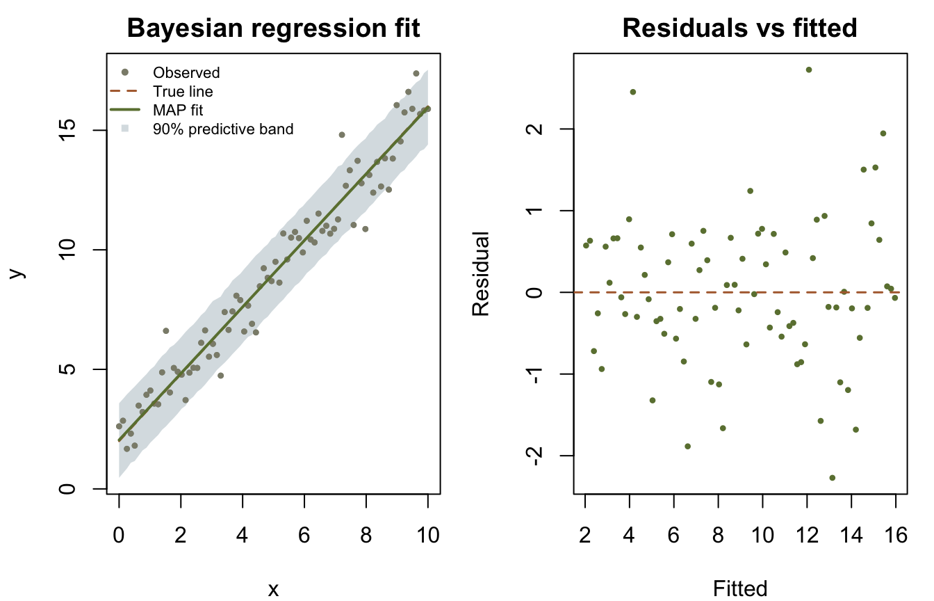
What the returned curves are, since they differ from the upstream plot:

• mode_curve is the deterministic fitted line \(\mu + \gamma t\) evaluated at the MAP parameters.
• mean_curve, lower_ci, and upper_ci come from a posterior predictive ensemble: each posterior draw simulates a full series including observation noise. The 90% band is therefore a predictive band for observations, wider than the mean-function credible band the upstream script plots.

The upstream 2x2 figure also shows posterior histograms of a, b, and sigma; the analysis returns curves and MAP values rather than raw chains, so those two panels cannot be reproduced here.

true_line <- true_a + true_b * x

op <- par(mfrow = c(1, 2), mar = c(4, 4, 2, 1))

plot(x, y,
  pch = 16, cex = 0.6, col = "#8c8c7a",
  ylim = range(fit$lower_ci, fit$upper_ci, y),
  xlab = "x", ylab = "y", main = "Bayesian regression fit"
)
polygon(c(x, rev(x)), c(fit$lower_ci, rev(fit$upper_ci)),
  col = adjustcolor("#5b7a8c", alpha.f = 0.25), border = NA
)
points(x, y, pch = 16, cex = 0.6, col = "#8c8c7a")
lines(x, true_line, col = "#b06a3b", lty = 2, lwd = 1.5)
lines(x, fit$mode_curve, col = "#6b7f3f", lwd = 2)
legend("topleft",
  legend = c("Observed", "True line", "MAP fit", "90% predictive band"),
  col = c("#8c8c7a", "#b06a3b", "#6b7f3f", adjustcolor("#5b7a8c", alpha.f = 0.25)),
  pch = c(16, NA, NA, 15), lty = c(NA, 2, 1, NA), lwd = c(NA, 1.5, 2, NA),
  bty = "n", cex = 0.7
)

residuals <- y - fit$mode_curve
plot(fit$mode_curve, residuals,
  pch = 16, cex = 0.6, col = "#6b7f3f",
  xlab = "Fitted", ylab = "Residual", main = "Residuals vs fitted"
)
abline(h = 0, col = "#b06a3b", lty = 2, lwd = 1.5)

par(op)

inside <- (y >= fit$lower_ci) & (y <= fit$upper_ci)
covers_true <- (true_line >= fit$lower_ci) & (true_line <= fit$upper_ci)
cat(sprintf("observations inside the 90%% predictive band: %.4f\n", mean(inside)))

observations inside the 90% predictive band: 0.8875

cat(sprintf("ordinates where the band covers the true line: %d of %d\n", sum(covers_true), n))

ordinates where the band covers the true line: 80 of 80

Reproduction check

The upstream file is a script with no committed outputs, so there are no upstream posterior literals to compare against; the reference values are the true generating parameters. The priors and the parameterization deliberately differ (data-scaled uniform priors, time-index trend), so bit-comparison with the upstream posterior is impossible and the parameter checks are statistical. The exact tier covers what is exactly checkable: the seeded synthetic data (the same Mersenne Twister stream the upstream draws) and cross-language identity of the whole analysis (the Python twin asserts the same MAP literals from the same seed).

Quantity	Upstream C#	This port	Status
Seeded data y[1] (seed 123)	same MT stream	2.61712675977869	exact
Seeded data y[80]	same MT stream	15.89237584375904	exact
Intercept a	2.0 (true)	MAP 2.0437	statistical
Slope b	1.4 (true)	MAP 1.3916	statistical
sigma	1.2 nominal, 0.9037 realized	MAP 0.9185	statistical
90% band covers the true line	-	80 of 80 ordinates	statistical

The chunk below fails the render if any value drifts.

# Upstream: examples/bayesian_regression.py (a script with no committed outputs;
# the reference values are the true generating parameters, not upstream posteriors).

# Exact tier: seeded data and the fit itself, identical across R, Python, and the
# C# library. The values are bit-exact (the fixture suite enforces that); the
# comparisons carry a 1e-15 relative tolerance only because R's decimal parser can
# land one ulp away from the written literal.
stopifnot(
  abs(y[1] / 2.6171267597786905 - 1) < 1e-15,
  abs(y[n] / 15.892375843759043 - 1) < 1e-15,
  abs(mu_map / 2.043676501381344 - 1) < 1e-15,
  abs(gamma_map / 0.1761574955229039 - 1) < 1e-15
)

# Statistical tier: recovered parameters near the truth. Priors and parameterization
# deliberately differ from the upstream script, so only closeness can be asserted.
stopifnot(
  abs(mu_map - true_a) < 0.5,
  abs(b_map - true_b) < 0.1,
  sigma_map > 0.7, sigma_map < 1.2 # tracks the realized noise sd, 0.9037
)

# Statistical tier: the 90% predictive band covers the true line everywhere and
# most observations.
stopifnot(
  all(covers_true),
  mean(inside) > 0.8
)
cat("All reproduction checks passed.\n")

All reproduction checks passed.